## Rows: 53,940
## Columns: 10
## $ carat   <dbl> 0.23, 0.21, 0.23, 0.29, 0.31, 0.24, 0.24, 0.26, 0.22, 0.23, 0.…
## $ cut     <ord> Ideal, Premium, Good, Premium, Good, Very Good, Very Good, Ver…
## $ color   <ord> E, E, E, I, J, J, I, H, E, H, J, J, F, J, E, E, I, J, J, J, I,…
## $ clarity <ord> SI2, SI1, VS1, VS2, SI2, VVS2, VVS1, SI1, VS2, VS1, SI1, VS1, …
## $ depth   <dbl> 61.5, 59.8, 56.9, 62.4, 63.3, 62.8, 62.3, 61.9, 65.1, 59.4, 64…
## $ table   <dbl> 55, 61, 65, 58, 58, 57, 57, 55, 61, 61, 55, 56, 61, 54, 62, 58…
## $ price   <int> 326, 326, 327, 334, 335, 336, 336, 337, 337, 338, 339, 340, 34…
## $ x       <dbl> 3.95, 3.89, 4.05, 4.20, 4.34, 3.94, 3.95, 4.07, 3.87, 4.00, 4.…
## $ y       <dbl> 3.98, 3.84, 4.07, 4.23, 4.35, 3.96, 3.98, 4.11, 3.78, 4.05, 4.…
## $ z <dbl> 2.43, 2.31, 2.31, 2.63, 2.75, 2.48, 2.47, 2.53, 2.49, 2.39, 2.…206 Question
Schlüsselwörter
Aufgaben, Statistik, Prognose, Modellierung, R, Datenanalyse, Regression
In dieser Aufgaben analysieren wir den Datensatz diamonds, welcher Merkmale von Diamanten (wie Preis, Schliffart etc.) auflistet. Hier ist ein Blick in den Datensatz:
diamonds ist Teil von Tidyverse (genauer gesagt dem Paket ggplot2).
Hier ist ein Überblick über die deskriptiven, univariaten Statistiken:
| Name | diamonds |
| Number of rows | 53940 |
| Number of columns | 10 |
| _______________________ | |
| Column type frequency: | |
| factor | 3 |
| numeric | 7 |
| ________________________ | |
| Group variables | None |
Variable type: factor
| skim_variable | n_missing | complete_rate | ordered | n_unique | top_counts |
|---|---|---|---|---|---|
| cut | 0 | 1 | TRUE | 5 | Ide: 21551, Pre: 13791, Ver: 12082, Goo: 4906 |
| color | 0 | 1 | TRUE | 7 | G: 11292, E: 9797, F: 9542, H: 8304 |
| clarity | 0 | 1 | TRUE | 8 | SI1: 13065, VS2: 12258, SI2: 9194, VS1: 8171 |
Variable type: numeric
| skim_variable | n_missing | complete_rate | mean | sd | p0 | p25 | p50 | p75 | p100 | hist |
|---|---|---|---|---|---|---|---|---|---|---|
| carat | 0 | 1 | 0.80 | 0.47 | 0.2 | 0.40 | 0.70 | 1.04 | 5.01 | ▇▂▁▁▁ |
| depth | 0 | 1 | 61.75 | 1.43 | 43.0 | 61.00 | 61.80 | 62.50 | 79.00 | ▁▁▇▁▁ |
| table | 0 | 1 | 57.46 | 2.23 | 43.0 | 56.00 | 57.00 | 59.00 | 95.00 | ▁▇▁▁▁ |
| price | 0 | 1 | 3932.80 | 3989.44 | 326.0 | 950.00 | 2401.00 | 5324.25 | 18823.00 | ▇▂▁▁▁ |
| x | 0 | 1 | 5.73 | 1.12 | 0.0 | 4.71 | 5.70 | 6.54 | 10.74 | ▁▁▇▃▁ |
| y | 0 | 1 | 5.73 | 1.14 | 0.0 | 4.72 | 5.71 | 6.54 | 58.90 | ▇▁▁▁▁ |
| z | 0 | 1 | 3.54 | 0.71 | 0.0 | 2.91 | 3.53 | 4.04 | 31.80 | ▇▁▁▁▁ |
Betrachten Sie das Histogramm; welcher R-Code hat es erzeugt?
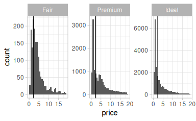
Für alle Diagramme gilt:
A
diamonds %>%
  mutate(price = price/1000 %>% round) %>%
  ggplot() +
  aes(x = price) +
  geom_histogram()  +
  geom_vline(aes(xintercept = mean(price))) +
  theme_light() +
  facet_wrap( ~ cut, scales = "free")
B
diamonds %>%
  drop_na(cut, price) %>%
  filter(cut %in% c("Fair", "Premium", "Ideal")) %>%
  mutate(price = price/1000 %>% round) %>%
  ggplot() +
  aes(x = price) +
  geom_histogram()  +
  geom_vline(aes(xintercept = median(price))) +
  theme_light() +
  facet_wrap( ~ cut, scales = "free")
C
diamonds %>%
  drop_na(cut, price) %>%
  filter(cut %in% c("Fair", "Premium", "Ideal")) %>%
  ggplot() +
  aes(x = price) +
  geom_histogram()  +
  geom_vline(aes(xintercept = median(price)))
  facet_wrap(cut)
D
diamonds %>%
  drop_na(cut, price) %>%
  filter(cut %in% c("Fair", "Premium", "Ideal")) %>%
  ggplot() +
  aes(x = price) +
  geom_histogram()  +
  geom_vline(aes(xintercept = median(price))) +
  theme_light() +
  facet_wrap( ~ cut, scales = "free")
206.1 Answerlist
- Code-Beispiel A
- Code-Beispiel B
- Code-Beispiel C
- Code-Beispiel D
- Keine Antwort möglich
207 Solution
Code B passt zum Diagramm.
207.1 Answerlist
- Falsch
- Richtig
- Falsch
- Falsch
- Falsch
208 Meta-information
exname: diamonds-histogram-rcode extype: schoice exsolution: 01000 exshuffle: TRUE expoints: 1