90  nichtlineare-regr1

Schlüsselwörter

Aufgaben, Statistik, Prognose, Modellierung, R, Datenanalyse, Regression

90.1 Aufgabe

Wir suchen ein Modell, das einen nichtlinearen Zusammenhang von PS-Zahl und Spritverbrauch darstellt (Datensatz mtcars).

Geben Sie dafür ein mögliches Modell an! Nutzen Sie den R-Befehl lm.

90.2 Lösung

mtcars <-
  mtcars %>% 
  mutate(mpg_log = log(mpg)) 

lm1 <- lm(mpg_log ~ hp, data = mtcars)
summary(lm1)
## 
## Call:
## lm(formula = mpg_log ~ hp, data = mtcars)
## 
## Residuals:
##      Min       1Q   Median       3Q      Max 
## -0.41577 -0.06583 -0.01737  0.09827  0.39621 
## 
## Coefficients:
##               Estimate Std. Error t value Pr(>|t|)    
## (Intercept)  3.4604669  0.0785838  44.035  < 2e-16 ***
## hp          -0.0034287  0.0004867  -7.045 7.85e-08 ***
## ---
## Signif. codes:  0 '***' 0.001 '**' 0.01 '*' 0.05 '.' 0.1 ' ' 1
## 
## Residual standard error: 0.1858 on 30 degrees of freedom
## Multiple R-squared:  0.6233, Adjusted R-squared:  0.6107 
## F-statistic: 49.63 on 1 and 30 DF,  p-value: 7.853e-08

Visualisieren wir die Vorhersagen des Modells:

mtcars <-
  mtcars %>% 
  mutate(pred = predict(lm1))

mtcars %>% 
  ggplot() +
  aes(x = hp) +
  geom_line(aes( y = pred), color = "blue") +
  geom_point(aes(y = mpg_log)) +
  labs(y = "log(mpg)",
       title = "Vorhersage von log-mpg in einem Log-Y-Modell")

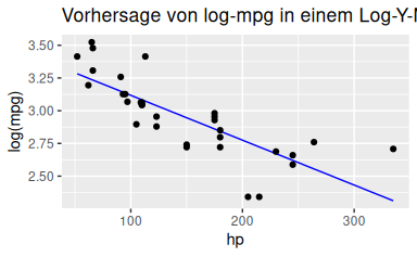
Oder so visualisieren:

library(easystats)
# estimate_expectation(lm1, by = "hp") %>% plot()

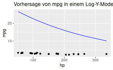
Möchte man auf der Y-Achse mpg und nicht log(mpg) anzeigen, muss man den Logarithmus wieder “auflösen”, das erreicht man mit der Umkehrfunktion des Logarithmus, das Exponentieren (man “delogarithmiert”):

\[\begin{aligned} log(y) &= x \qquad | \text{Y in Log-Form}\\ exp(log(y)) &= exp(x) \qquad | \text{Jetzt exponenzieren wir beide Seiten}\\ y = exp(x) \end{aligned}\]

Dabei gilt \(exp(x) = e^x\), mit \(e\) als Eulersche Zahl (2.71828…).

mtcars <-
  mtcars %>% 
  mutate(pred_delog = exp(pred))  # delogarithmieren

mtcars %>% 
  ggplot() +
  aes(x = hp) +
  geom_line(aes( y = pred_delog), color = "blue") +
  geom_point(aes(y = mpg_log)) +
  labs(y = "mpg",
       title = "Vorhersage von mpg in einem Log-Y-Modell")

---

Categories:

• lm
• vis
• qm2
• regression
• string