8 KI-Gebrauch
8.1 Setup
Show the code
source("_common.r")Show the code
tar_load(
  c(
    ai_transcript_clicks_per_month,
    data_long,
    data_separated_distinct_slice,
    data_separated_filtered,
    idvisit_has_llm,
    llm_response_text,
    n_mc_answers_selected,
    mc_answers_with_timestamps,
    prompt_length,
    prompt_length_date_uni_course,
    time_spent_w_course_university,
    llm_response_text_date_course_uni,
    n_interactions_w_llm_course_date_course_uni
  )
)
8.2 Interaktion mit dem LLM
Berechnungsgrundlage: Für diese Analyse wurden alle Events der Kategorie llm gefiltert.
8.2.1 Art und Anzahl der Interaktionen mit dem LLM
Show the code
Show the code
data_separated_filtered_ai |>
  mutate(prop = round(prop, 3)) |>
  ggtexttable()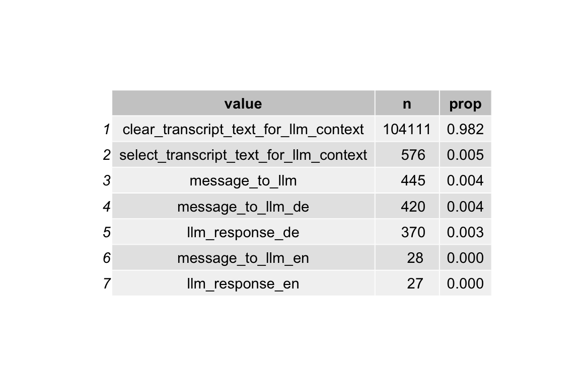
8.3 Anzahl der message_to_llm
Show the code
llm_interactions <-
  data_separated_filtered |>
  filter(str_detect(value, "message_to_llm"))
8.3.1 Verteilung
Show the code
| Variable | Median | MAD | Mean | SD | IQR | Range | Skewness | Kurtosis | n | n_Missing |
|---|---|---|---|---|---|---|---|---|---|---|
| messages_to_llm_n | 6 | 2.97 | 9.65 | 8.22 | 8 | (2.00, 44.00) | 1.86 | 3.71 | 185 | 0 |
8.3.2 Diagramm
Show the code
gghistogram(
  llm_interactions_count,
  x = "messages_to_llm_n",
  bins = 10,
  add = "median"
) +
  labs(caption = "The vertical dotted line denotes the median.")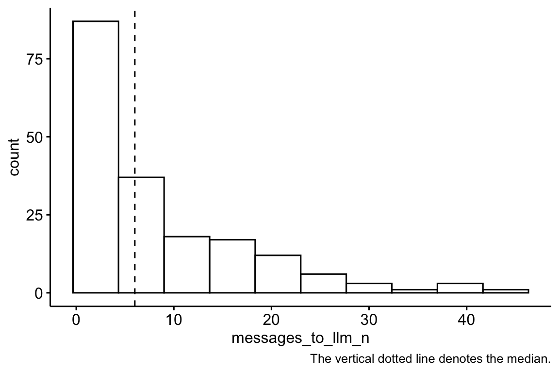
8.4 Anteil Visitors, die mit dem LLM interagieren
8.4.1 idvisit
Show the code
data_separated_filtered_llm_interact <-
  data_separated_filtered |>
  mutate(has_llm = str_detect(value, "llm")) |>
  group_by(idvisit) |>
  summarise(llm_used_during_visit = any(has_llm == TRUE)) |>
  count(llm_used_during_visit) |>
  mutate(prop = round(n / sum(n), 2))

data_separated_filtered_llm_interact |>
gt()| llm_used_during_visit | n | prop |
|---|---|---|
| FALSE | 13419 | 0.94 |
| TRUE | 788 | 0.06 |
Show the code
data_separated_filtered_llm_interact |>
  ggtexttable()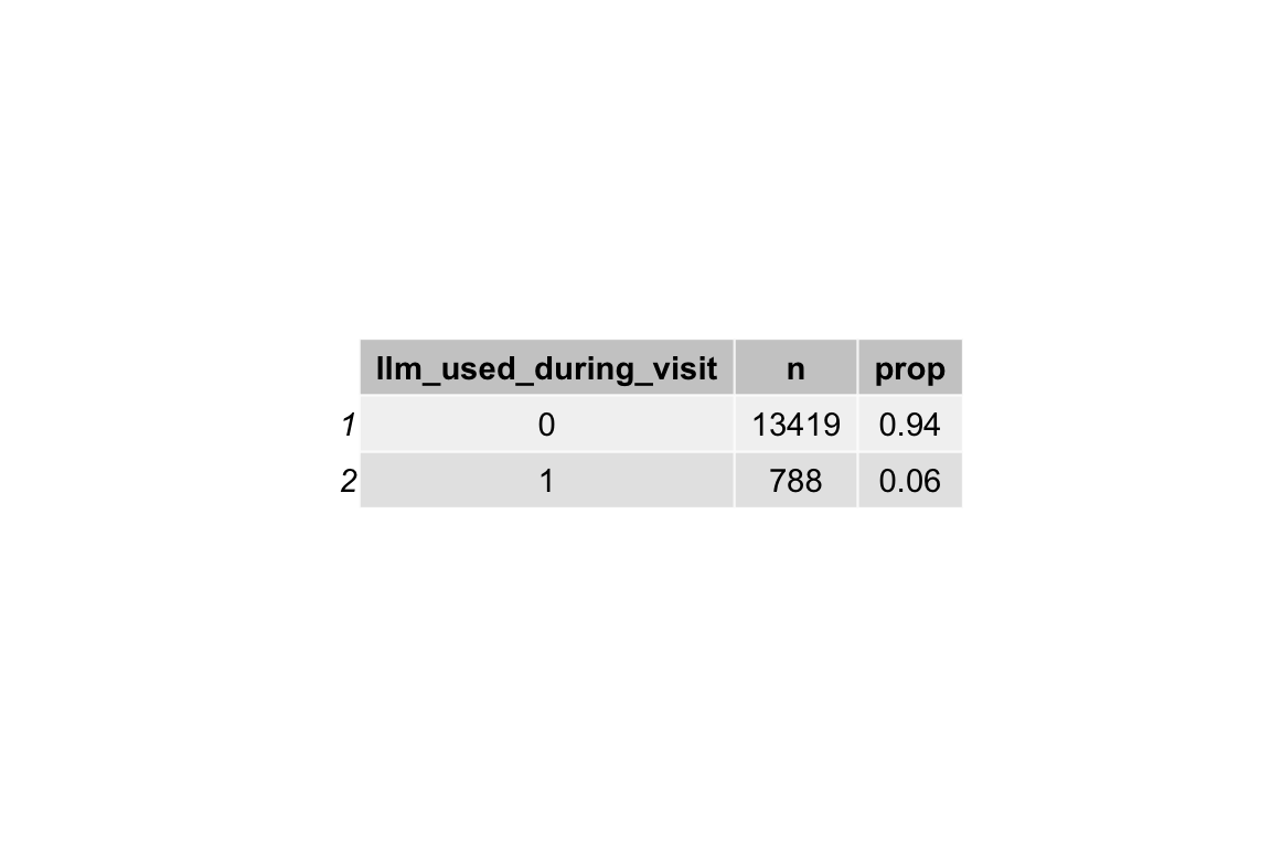
8.4.2 fingerprint unique
Show the code
data_separated_filtered_llm_interact_fingerprint <-
  data_separated_filtered |>
  mutate(has_llm = str_detect(value, "llm")) |>
  group_by(fingerprint) |>
  summarise(llm_used_during_visit = any(has_llm == TRUE)) |>
  count(llm_used_during_visit) |>
  mutate(prop = round(n / sum(n), 2))

data_separated_filtered_llm_interact_fingerprint |>
gt()| llm_used_during_visit | n | prop |
|---|---|---|
| FALSE | 6649 | 0.93 |
| TRUE | 511 | 0.07 |
Show the code
data_separated_filtered_llm_interact_fingerprint |>
  ggtexttable()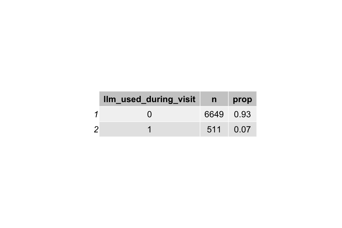
8.4.3 … Im Zeitverlauf
8.4.3.1 Absolutzahlen
Show the code
idvisit_has_llm |>
  head(30)
Show the code
Show the code
idvisit_has_llm_timeline |>
  ggtexttable()
Show the code
idvisit_has_llm |>
  count(year_month, uses_llm) |>
  ungroup() |>
  mutate(year_month_date = ymd(paste0(year_month, "-01"))) |>
  group_by(year_month_date) |>
  mutate(prop = n / sum(n)) |>
  ggplot(aes(
    x = year_month_date,
    y = prop,
    color = uses_llm,
    groups = uses_llm
  )) +
  # --- Highlight March–July (approx 1 Mar to 31 Jul) ---
  annotate(
    "rect",
    xmin = as.Date("2023-03-01"),
    xmax = as.Date("2023-07-31"),
    ymin = -Inf,
    ymax = Inf,
    alpha = 0.2,
    fill = "skyblue"
  ) +

  annotate(
    "rect",
    xmin = as.Date("2024-03-01"),
    xmax = as.Date("2024-07-31"),
    ymin = -Inf,
    ymax = Inf,
    alpha = 0.2,
    fill = "skyblue"
  ) +
  annotate(
    "rect",
    xmin = as.Date("2025-03-01"),
    xmax = as.Date("2025-07-31"),
    ymin = -Inf,
    ymax = Inf,
    alpha = 0.2,
    fill = "skyblue"
  ) +

  # --- Highlight October–February (semester break or 2nd term) ---
  annotate(
    "rect",
    xmin = as.Date("2023-10-01"),
    xmax = as.Date("2024-02-28"),
    ymin = -Inf,
    ymax = Inf,
    alpha = 0.2,
    fill = "orange"
  ) +
  # annotate("rect",
  #          xmin = as.Date("2024-10-01"), xmax = as.Date("2024-02-28"),
  #          ymin = -Inf, ymax = Inf, alpha = 0.2, fill = "orange") +
  annotate(
    "rect",
    xmin = as.Date("2024-10-01"),
    xmax = as.Date("2025-02-28"),
    ymin = -Inf,
    ymax = Inf,
    alpha = 0.2,
    fill = "orange"
  ) +
  geom_point() +
  geom_line(aes(group = uses_llm)) +
  labs(
    title = "Visitors, die mit dem LLM interagieren im Zeitverlauf (Anteile)"
  ) +
  scale_x_date(breaks = pretty_breaks())
Show the code
idvisit_has_llm |>
  count(year_month, uses_llm) |>
  ungroup() |>
  mutate(year_month_date = ymd(paste0(year_month, "-01"))) |>
  group_by(year_month) |>
  ggplot(aes(x = year_month_date, y = n, color = uses_llm, groups = uses_llm)) +
  # --- Highlight March–July (approx 1 Mar to 31 Jul) ---
  annotate(
    "rect",
    xmin = as.Date("2023-03-01"),
    xmax = as.Date("2023-07-31"),
    ymin = -Inf,
    ymax = Inf,
    alpha = 0.2,
    fill = "skyblue"
  ) +

  annotate(
    "rect",
    xmin = as.Date("2024-03-01"),
    xmax = as.Date("2024-07-31"),
    ymin = -Inf,
    ymax = Inf,
    alpha = 0.2,
    fill = "skyblue"
  ) +
  annotate(
    "rect",
    xmin = as.Date("2025-03-01"),
    xmax = as.Date("2025-07-31"),
    ymin = -Inf,
    ymax = Inf,
    alpha = 0.2,
    fill = "skyblue"
  ) +

  # --- Highlight October–February (semester break or 2nd term) ---
  annotate(
    "rect",
    xmin = as.Date("2023-10-01"),
    xmax = as.Date("2024-02-28"),
    ymin = -Inf,
    ymax = Inf,
    alpha = 0.2,
    fill = "orange"
  ) +
  # annotate("rect",
  #          xmin = as.Date("2024-10-01"), xmax = as.Date("2024-02-28"),
  #          ymin = -Inf, ymax = Inf, alpha = 0.2, fill = "orange") +
  annotate(
    "rect",
    xmin = as.Date("2024-10-01"),
    xmax = as.Date("2025-02-28"),
    ymin = -Inf,
    ymax = Inf,
    alpha = 0.2,
    fill = "orange"
  ) +
  geom_point() +
  geom_line(aes(group = uses_llm)) +
  labs(
    title = "Visitors, die mit dem LLM interagieren im Zeitverlauf (Anzahl)"
  ) +
  scale_x_date(breaks = pretty_breaks())
8.4.3.2 Anteile
Show the code
idvisit_has_llm |>
  count(year_month, uses_llm) |>
  ungroup() |>
  mutate(year_month_date = ymd(paste0(year_month, "-01"))) |>
  group_by(year_month_date) |>
  # ADDED: Calculate the proportion
  mutate(proportion = n / sum(n)) |>

  # Plot using the new 'proportion' variable
  ggplot(aes(x = year_month_date, y = proportion, fill = uses_llm)) +

  # ADDED: Use position = "fill"
  geom_area(position = "fill") +

  # ADDED: Format y-axis as percentage
  scale_y_continuous(labels = scales::label_percent()) +

  labs(
    title = "Anteil der Besucher, die mit dem LLM interagieren (Prozent)",
    y = "Prozentualer Anteil der Besucher",
    fill = "Interagiert mit LLM",
    x = "Datum"
  ) +
  scale_x_date(breaks = pretty_breaks())
8.5 Länge der Prompts (Input an das LLM)
8.5.1 Überblick
Show the code
prompt_length_no_prompts |>
  describe_distribution(token_length) |>
print_md()| Variable | Mean | SD | IQR | Range | Skewness | Kurtosis | n | n_Missing |
|---|---|---|---|---|---|---|---|---|
| token_length | 6.86 | 6.16 | 4 | (1.00, 79.00) | 4.76 | 43.63 | 893 | 0 |
Show the code
prompt_length_no_prompts |>
  ggplot(aes(x = token_length)) +
  geom_histogram(binwidth = 10) +
  labs(
    title = "Length of prompts sent to the LLM",
    x = "Prompt length (in tokens)",
    y = "Number of prompts"
  ) +
  theme_minimal()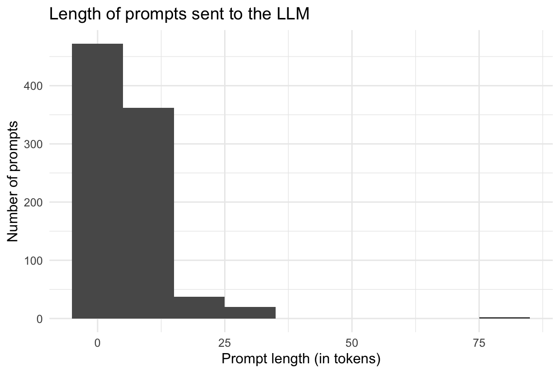
Show the code
describe_distribution(
  prompt_length$prompt_length,
  centrality = c("mean", "median")
)NULL8.5.2 Token-Länge nach Universitäten
Show the code
| university | Variable | Mean | SD | IQR | Range | Skewness | Kurtosis | n | n_Missing |
|---|---|---|---|---|---|---|---|---|---|
| evhn | token_length | (Inf, -Inf) | 0 | 6 | |||||
| hnu | token_length | 7.00 | 0.00 | 0 | (7.00, 7.00) | 6 | 12 | ||
| hs-ansbach | token_length | (Inf, -Inf) | 0 | 3 | |||||
| hswt | token_length | 6.54 | 4.08 | 9 | (1.00, 12.00) | -0.15 | -1.47 | 48 | 1094 |
| iqw | token_length | (Inf, -Inf) | 0 | 1 | |||||
| th-nuernberg | token_length | 8.11 | 9.20 | 8 | (1.00, 79.00) | 4.38 | 28.22 | 246 | 4224 |
| th-owl | token_length | (Inf, -Inf) | 0 | 1 | |||||
| thi | token_length | 10.00 | 10.03 | 18 | (2.00, 26.00) | 1.31 | -0.14 | 8 | 438 |
Show the code
ggboxplot(
  prompt_length_date_uni_course,
  x = "university",
  y = "token_length",
  add = "mean_se",
) +
  theme_minimal() +
  labs(
    title = "Prompt length by university",
    x = "University",
    y = "Prompt length (in tokens)"
  ) +
  coord_flip()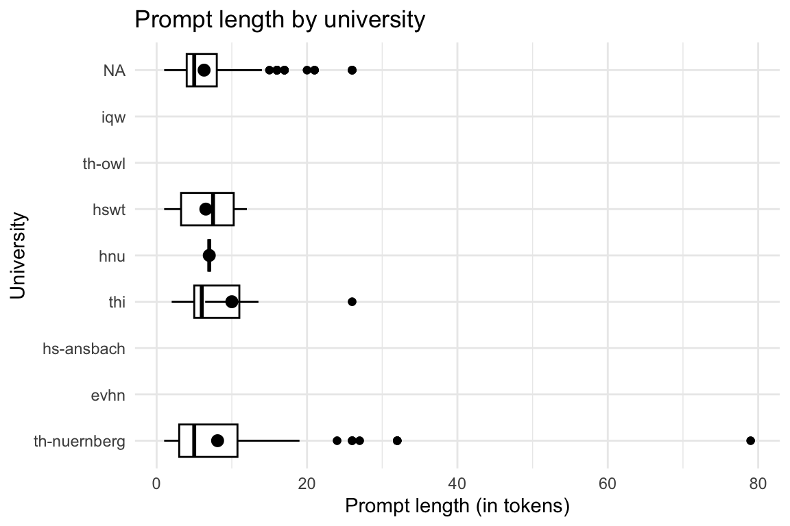
8.5.3 Token-Länge nach Kursen
Show the code
| course | Variable | Mean | SD | IQR | Range | Skewness | Kurtosis | n | n_Missing |
|---|---|---|---|---|---|---|---|---|---|
| anis2 | token_length | (Inf, -Inf) | 0 | 43 | |||||
| armeufa | token_length | (Inf, -Inf) | 0 | 2 | |||||
| bare | token_length | 7.00 | 0.00 | 0 | (7.00, 7.00) | 6 | 12 | ||
| bio | token_length | (Inf, -Inf) | 0 | 168 | |||||
| biotech | token_length | (Inf, -Inf) | 0 | 127 | |||||
| biovete | token_length | (Inf, -Inf) | 0 | 244 | |||||
| cta1 | token_length | 6.54 | 4.08 | 9 | (1.00, 12.00) | -0.15 | -1.47 | 48 | 1094 |
| daba | token_length | 5.00 | 0.00 | 0 | (5.00, 5.00) | 2 | 197 | ||
| enerbi | token_length | (Inf, -Inf) | 0 | 10 | |||||
| epsy | token_length | (Inf, -Inf) | 0 | 1 | |||||
| etechde | token_length | (Inf, -Inf) | 0 | 3 | |||||
| fodesoa | token_length | 3.00 | 0.00 | 0 | (3.00, 3.00) | 2 | 324 | ||
| fomesoa | token_length | (Inf, -Inf) | 0 | 6 | |||||
| fosaq | token_length | 4.00 | 0.00 | 0 | (4.00, 4.00) | 2 | 59 | ||
| gdi | token_length | 7.67 | 2.88 | 6 | (4.00, 10.00) | -0.86 | -1.88 | 6 | 47 |
| gemwesa | token_length | (Inf, -Inf) | 0 | 57 | |||||
| gesoa | token_length | 6.67 | 9.64 | 4 | (1.00, 79.00) | 5.88 | 41.54 | 150 | 2315 |
| kore | token_length | (Inf, -Inf) | 0 | 3 | |||||
| mat11akzg | token_length | (Inf, -Inf) | 0 | 2 | |||||
| mibio | token_length | (Inf, -Inf) | 0 | 206 | |||||
| mioek | token_length | 10.00 | 10.03 | 18 | (2.00, 26.00) | 1.31 | -0.14 | 8 | 435 |
| nlp | token_length | 8.00 | 3.46 | 6 | (5.00, 11.00) | 0.00 | -6.00 | 4 | 65 |
| quame1 | token_length | (Inf, -Inf) | 0 | 3 | |||||
| quanch | token_length | (Inf, -Inf) | 0 | 34 | |||||
| softa | token_length | (Inf, -Inf) | 0 | 4 | |||||
| thesoa | token_length | 11.15 | 8.45 | 8 | (1.00, 32.00) | 1.29 | 0.97 | 80 | 272 |
| wirkori | token_length | (Inf, -Inf) | 0 | 5 | |||||
| wisoa | token_length | (Inf, -Inf) | 0 | 33 | |||||
| zemiws | token_length | (Inf, -Inf) | 0 | 1 |
Show the code
ggboxplot(
  prompt_length_date_uni_course,
  x = "course",
  y = "token_length",
  add = "mean_se",
) +
  theme_minimal() +
  labs(
    title = "Prompt length by course",
    x = "Course",
    y = "Prompt length (in tokens)"
  ) +
  coord_flip()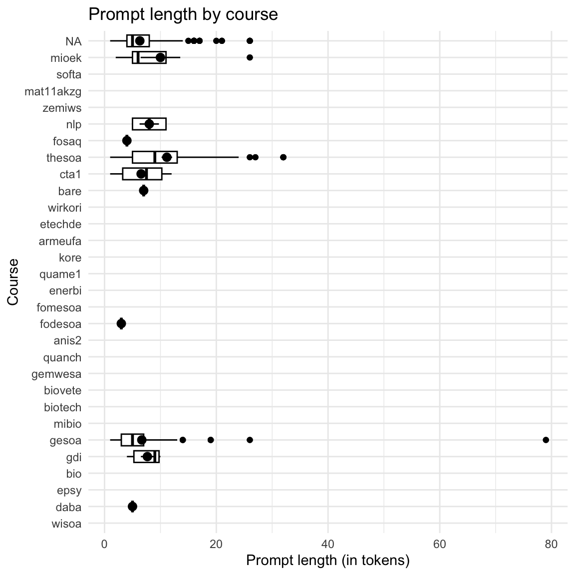
8.5.4 Token-Länge im Zeitverlauf
Show the code
| floor_date_month | Variable | Mean | SD | IQR | Range | Skewness | Kurtosis | n | n_Missing |
|---|---|---|---|---|---|---|---|---|---|
| 2022-12-01 | token_length | (Inf, -Inf) | 0 | 329 | |||||
| 2023-01-01 | token_length | (Inf, -Inf) | 0 | 455 | |||||
| 2023-02-01 | token_length | (Inf, -Inf) | 0 | 561 | |||||
| 2023-03-01 | token_length | (Inf, -Inf) | 0 | 149 | |||||
| 2023-04-01 | token_length | (Inf, -Inf) | 0 | 253 | |||||
| 2023-05-01 | token_length | (Inf, -Inf) | 0 | 391 | |||||
| 2023-06-01 | token_length | (Inf, -Inf) | 0 | 292 | |||||
| 2023-07-01 | token_length | (Inf, -Inf) | 0 | 441 | |||||
| 2023-08-01 | token_length | (Inf, -Inf) | 0 | 26 | |||||
| 2023-09-01 | token_length | (Inf, -Inf) | 0 | 39 | |||||
| 2023-10-01 | token_length | (Inf, -Inf) | 0 | 614 | |||||
| 2023-11-01 | token_length | 5.57 | 5.56 | 7.00 | (1.00, 17.00) | 1.77 | 3.36 | 7 | 656 |
| 2023-12-01 | token_length | (Inf, -Inf) | 0 | 519 | |||||
| 2024-01-01 | token_length | 6.67 | 1.15 | 2.00 | (6.00, 8.00) | 1.73 | -1.50 | 3 | 781 |
| 2024-02-01 | token_length | (Inf, -Inf) | 0 | 85 | |||||
| 2024-03-01 | token_length | 5.54 | 2.47 | 1.00 | (2.00, 13.00) | 2.25 | 5.41 | 26 | 133 |
| 2024-04-01 | token_length | 5.33 | 1.67 | 2.00 | (2.00, 9.00) | 0.15 | 0.44 | 30 | 322 |
| 2024-05-01 | token_length | 3.57 | 1.81 | 4.00 | (1.00, 5.00) | -0.98 | -1.08 | 7 | 410 |
| 2024-06-01 | token_length | 8.16 | 5.82 | 9.00 | (1.00, 26.00) | 1.15 | 1.25 | 106 | 571 |
| 2024-07-01 | token_length | 7.14 | 6.07 | 13.00 | (3.00, 16.00) | 1.21 | -0.86 | 7 | 740 |
| 2024-08-01 | token_length | (Inf, -Inf) | 0 | 16 | |||||
| 2024-09-01 | token_length | 6.12 | 3.00 | 5.00 | (4.00, 11.00) | 0.82 | -1.49 | 8 | 21 |
| 2024-10-01 | token_length | 7.26 | 11.67 | 4.00 | (1.00, 79.00) | 4.94 | 27.91 | 100 | 714 |
| 2024-11-01 | token_length | 4.46 | 2.44 | 3.00 | (1.00, 12.00) | 0.88 | 1.11 | 76 | 900 |
| 2024-12-01 | token_length | 6.54 | 6.18 | 4.00 | (2.00, 26.00) | 2.64 | 6.71 | 26 | 759 |
| 2025-01-01 | token_length | 8.19 | 6.83 | 8.00 | (1.00, 32.00) | 2.16 | 4.85 | 148 | 936 |
| 2025-02-01 | token_length | 4.90 | 1.74 | 2.00 | (2.00, 8.00) | 0.17 | -0.44 | 20 | 152 |
| 2025-03-01 | token_length | 8.03 | 5.88 | 8.00 | (1.00, 21.00) | 0.79 | -0.36 | 62 | 490 |
| 2025-04-01 | token_length | 6.16 | 3.68 | 4.00 | (1.00, 17.00) | 0.77 | 0.24 | 191 | 978 |
| 2025-05-01 | token_length | 6.38 | 2.77 | 5.00 | (3.00, 11.00) | 0.26 | -1.47 | 37 | 546 |
| 2025-06-01 | token_length | 8.72 | 6.69 | 3.00 | (1.00, 26.00) | 1.33 | 1.77 | 29 | 315 |
| 2025-07-01 | token_length | 6.20 | 2.62 | 2.50 | (4.00, 11.00) | 1.50 | 0.86 | 10 | 427 |
Show the code
# Calculate limits properly
filtered_data <- prompt_length_date_uni_course |>
  filter(!is.na(floor_date_month)) |>
  mutate(floor_date_month_date = as.Date(floor_date_month))

lim <- c(
  min(filtered_data$floor_date_month_date, na.rm = TRUE),
  max(filtered_data$floor_date_month_date, na.rm = TRUE)
)

# Now create the plot
filtered_data |>
  ggplot(aes(x = floor_date_month_date, y = token_length)) +
  geom_violin(aes(group = floor_date_month_date)) +
  stat_summary(fun = "mean", geom = "point") +
  stat_summary(fun.data = "mean_se", geom = "errorbar", width = 0.2) +
  theme_minimal() +
  labs(
    title = "Prompt length over time",
    x = "Date",
    y = "Prompt length (in tokens)",
    caption = "The dots represent the mean and the error bars the standard error of the mean."
  ) +
scale_x_date(limits = lim, labels = scales::label_date_short()) 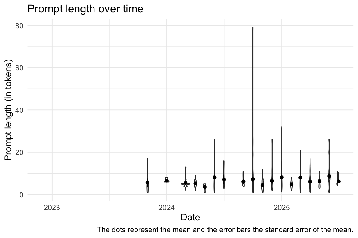
8.6 Anzahl der Interaktionen bei den Usern, die mit dem LLM interagieren
8.6.1 Insgesamt
Show the code
| Variable | Mean | SD | IQR | Range | Skewness | Kurtosis | n | n_Missing |
|---|---|---|---|---|---|---|---|---|
| n_interactions_w_llm | 165.59 | 216.45 | 459 | (1.00, 500.00) | 0.69 | -1.46 | 640 | 0 |
Show the code
d_n_interactions_w_llm |>
  ggplot(aes(x = n_interactions_w_llm)) +
  geom_histogram()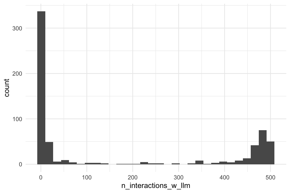
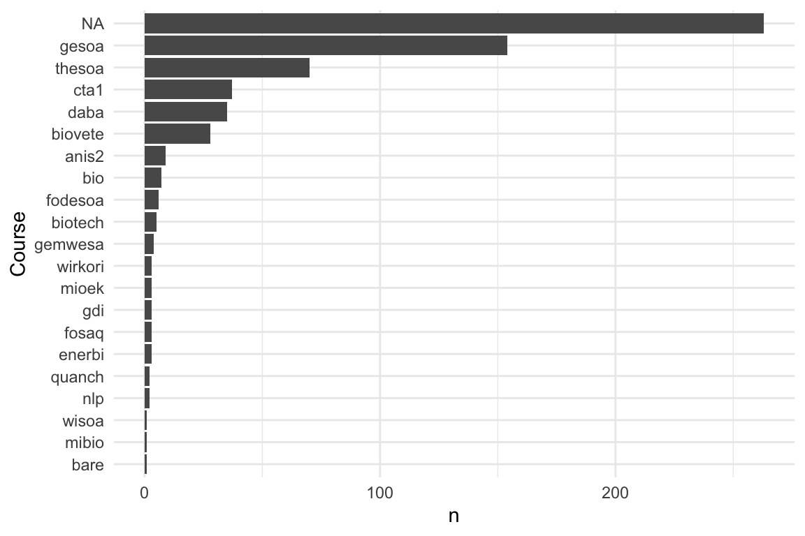
8.6.2 Interaktionen mit dem LLM - pro Kurs und pro Uni
Show the code
8.6.3 Interaktionen mit dem LLM - im Zeitverlauf
Show the code
rect_data <- comp_semester_rects(
  n_interactions_w_llm_course_date_course_uni,
  col_date = "floor_date_month"
)

n_interactions_w_llm_course_date_course_uni |>
  group_by(floor_date_month) |>
  summarise(n = n()) |>
  ggplot(aes(x = floor_date_month, y = n)) +
  geom_rect(
    data = rect_data,
    aes(xmin = xmin, xmax = xmax, ymin = ymin, ymax = ymax),
    fill = "grey",
    alpha = 0.2,
    inherit.aes = FALSE # Essential to use the rect_data columns
  ) +
  geom_line() +
labs(x = "Date", y = "Number of interactions with LLM") 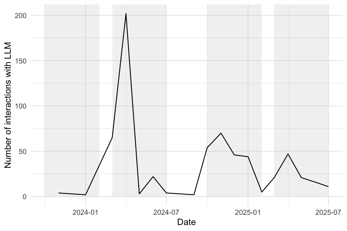
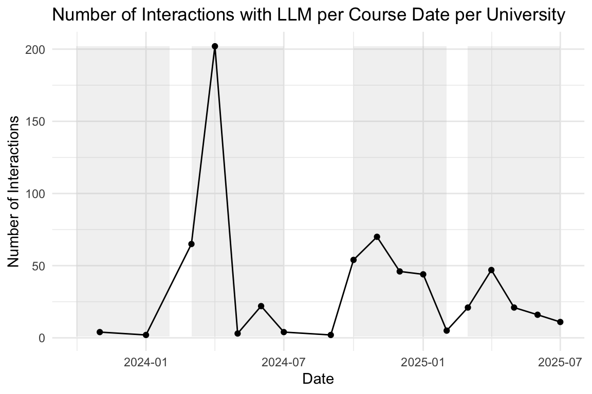
Show the code
# --- 1. Prepare Data ---
# Your original data processing for the plot
plot_data <- n_interactions_w_llm_course_date_course_uni |>
  group_by(floor_date_month) |>
  summarise(n = n()) |>
  ungroup() # Ungroup after summarise for easier use with ggplot

# --- 2. Determine Plot Range for Rectangles ---
# Find the min/max year and n-count from your *processed* plot_data
min_date <- min(plot_data$floor_date_month, na.rm = TRUE)
max_date <- max(plot_data$floor_date_month, na.rm = TRUE)
min_year <- year(min_date)
max_year <- year(max_date)

# Determine the Y-axis bounds for the rectangles
y_min <- min(plot_data$n, na.rm = TRUE)
y_max <- max(plot_data$n, na.rm = TRUE)

# --- 3. Calculate the Rectangle Coordinates (rect_data) ---

# Generate years for the rectangles, ensuring we cover the full range
# including potentially starting a "winter" semester in the min_year-1
# and ending in max_year+1
rect_years <- seq(min_year - 1, max_year + 1)

# Summer semester: March 1 (Y) to July 1 (Y)
summer_rects <- tibble(year = rect_years) |>
  mutate(
    xmin = ymd(paste0(year, "-03-01")),
    xmax = ymd(paste0(year, "-07-01"))
  )

# Winter semester: October 1 (Y) to February 1 (Y+1)
winter_rects <- tibble(year = rect_years) |>
  mutate(
    xmin = ymd(paste0(year, "-10-01")),
    xmax = ymd(paste0(year + 1, "-02-01"))
  )

# Combine, set Y bounds, and filter to the actual plot area
rect_data <- bind_rows(summer_rects, winter_rects) |>
  mutate(ymin = y_min, ymax = y_max) |>
  # Only keep rectangles that are fully or partially within the plot's X range
  filter(
    xmin <= max_date,
    xmax >= min_date
  )

# --- 4. Generate the Final Plot ---
plot_data |>
  ggplot(aes(x = floor_date_month, y = n)) +
  # Add the transparent grey rectangles first
  geom_rect(
    data = rect_data,
    aes(xmin = xmin, xmax = xmax, ymin = ymin, ymax = ymax),
    fill = "grey",
    alpha = 0.2,
    inherit.aes = FALSE # Essential to use the rect_data columns
  ) +
  # Then plot the lines and points on top
  geom_line() +
  geom_point() + # Added point layer for clarity at each month
  theme_minimal() +
  labs(
    title = "Number of Interactions with LLM per Course Date per University",
    x = "Date",
    y = "Number of Interactions"
) 
8.7 Klick auf ein Wort im Transkript
Ausgewertet wird im Folgenden die Variable “click_transcript_word”.
8.7.1 Insgesamt
Show the code
| click_transcript_word | n | prop |
|---|---|---|
| FALSE | 1138774 | 0.99 |
| TRUE | 8439 | 0.01 |
8.7.2 Im Zeitverlauf
8.7.2.1 idvisit
Show the code
click_transcript_word_per_month <-
  data_separated_filtered |>
  # rm all groups WITHOUT "click_transcript_word":
  group_by(idvisit) |>
  filter(!any(value = str_detect(value, "click_transcript_word"))) |>
  ungroup() |>
  mutate(date_visit = ymd_hms(value)) |>
  mutate(month_visit = floor_date(date_visit, unit = "month")) |>
  drop_na(date_visit) |>
  group_by(idvisit) |>
  slice(1) |>
  ungroup() |>
  count(month_visit)

click_transcript_word_per_month
Show the code
rect_data_word_per_month <- comp_semester_rects(
  click_transcript_word_per_month,
  col_date = "month_visit"
)

click_transcript_word_per_month |>
  ggplot(aes(x = month_visit, y = n)) +
  geom_rect(
    data = rect_data,
    aes(xmin = xmin, xmax = xmax, ymin = ymin, ymax = Inf),
    fill = "grey",
    alpha = 0.2,
    inherit.aes = FALSE # Essential to use the rect_data columns
  ) +
  geom_line() +
  geom_smooth(method = "loess", se = FALSE, color = "blue", alpha = 0.7) +
scale_x_date(labels = scales::label_date_short())![]()
8.7.2.2 fingerprint unique
Show the code
click_transcript_word_per_month_fingerprint <-
  data_separated_filtered |>
  # rm all groups WITHOUT "click_transcript_word":
  group_by(fingerprint) |>
  filter(!any(value = str_detect(value, "click_transcript_word"))) |>
  ungroup() |>
  mutate(date_visit = ymd_hms(value)) |>
  mutate(month_visit = floor_date(date_visit, unit = "month")) |>
  drop_na(date_visit) |>
  group_by(fingerprint) |>
  slice(1) |>
  ungroup() |>
  count(month_visit)

click_transcript_word_per_month_fingerprint
Show the code
click_transcript_word_per_month_fingerprint |>
  ggplot(aes(x = month_visit, y = n)) +
  geom_rect(
    data = rect_data,
    aes(xmin = xmin, xmax = xmax, ymin = ymin, ymax = Inf),
    fill = "grey",
    alpha = 0.2,
    inherit.aes = FALSE # Essential to use the rect_data columns
  ) +
  geom_line() +
geom_smooth(method = "loess", se = FALSE, color = "blue", alpha = 0.7)![]()
8.8 KI-Aktionen
8.8.1 Insgesamt (ganzer Zeitraum)
Show the code
data_long |>
  head(300)
8.8.2 Im Detail
Show the code
regex_pattern <- "Category: \"(.*?)(?=', Action)"

# Explaining this regex_pattern:
# Find the literal string
# 1. `Category: ` (surrounded by quotation marks)
# 2. Capture any characters (.*?) that follow, non-greedily, until...
# 3. ...it encounters the literal sequence,  ` Action`) immediately after the captured string.

ai_actions_count <-
  data_long |>
  # slice(1:1000) |>
  filter(str_detect(value, "transcript")) |>
  mutate(category = str_extract(value, regex_pattern)) |>
  select(category) |>
  mutate(category = str_replace_all(category, "[\"']", "")) |>
  count(category, sort = TRUE)

ai_actions_count |>
tt()| category | n |
|---|---|
| NA | 217862 |
| Category: clear_transcript_text_for_llm_context | 104111 |
| Category: click_transcript_word | 8439 |
| Category: select_transcript_text_for_llm_context | 576 |
| Category: click_button | 43 |
| Category: llm_response_de | 3 |
| Category: llm_response_en | 3 |
8.8.3 KI-Klicks pro Monat
Im Objekt wird gezählt, wie oft der String "click_transcript_word" in den Daten (Langformat) gefunden wird, s. Target ai_transcript_clicks_per_month in der Targets-Pipeline.
Show the code
ai_transcript_clicks_per_month |>
  head(30)
Show the code
Show the code
ai_transcript_clicks_per_month_count |>
  ggtexttable()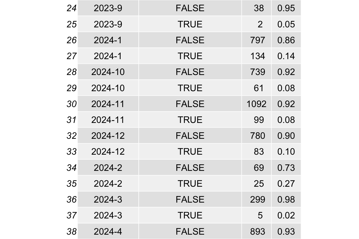
Show the code
rect_data <- comp_semester_rects(
  ai_transcript_clicks_per_month_count,
  col_date = "year_month"
)
# try common lubridate parsers (datetime -> date)

ai_transcript_clicks_per_month_count |>
  mutate(date = ymd(paste0(year_month, "-01"))) |>
  ggplot(aes(x = date, y = n)) +
  geom_rect(
    data = rect_data,
    aes(xmin = xmin, xmax = xmax, ymin = ymin, ymax = ymax),
    fill = "grey",
    alpha = 0.2,
    inherit.aes = FALSE # Essential to use the rect_data columns
  ) +
  geom_line(group = 1) +
  geom_point() +
  theme_minimal() +
  labs(
    title = "Number of AI transcript clicks per month",
    x = "date [months]"
  ) +
geom_smooth(method = "loess", se = FALSE, color = "blue", alpha = 0.2)![]()
Show the code
# --- 1. Prepare Data and Determine Year Range ---
# We assign the processed data to a temporary variable to calculate the year range.
ai_clicks_data <-
  ai_transcript_clicks_per_month_count |>
  mutate(date = ymd(paste0(year_month, "-01")))

# --- 2. Calculate the Vertical Line Intercept Dates ---
# Find the min/max year in the data
min_year <- min(year(ai_clicks_data$date), na.rm = TRUE)
max_year <- max(year(ai_clicks_data$date), na.rm = TRUE)
years <- seq(min_year, max_year)

# Define the target months: February (2), March (3), July (7), October (10)
vline_dates <- expand.grid(
  year = years,
  month = c(2, 3, 7, 10)
) |>
  mutate(
    date_str = paste0(year, "-", month, "-01"),
    vline_date = ymd(date_str)
  ) |>
  # Filter to only include dates within the actual data range for plotting
  filter(
    vline_date >= min(ai_clicks_data$date) &
      vline_date <= max(ai_clicks_data$date)
  ) |>
  pull(vline_date) |>
  as.Date()

# --- 3. Generate the Final Plot ---
ai_clicks_data |>
  ggplot(aes(x = date, y = n)) +
  # Add the vertical lines
  geom_vline(
    xintercept = vline_dates,
    color = "darkred",
    linetype = "dashed",
    alpha = 0.6
  ) +
  geom_line(group = 1) +
  geom_point() +
  theme_minimal() +
  labs(title = "Number of AI transcript clicks per month", x = "date [months]") +
geom_smooth(method = "loess", se = FALSE, color = "blue", alpha = 0.5)![]()
Show the code
# --- 1. Prepare Data and Determine Year Range ---
# We assign the processed data to a temporary variable to calculate the year range.
ai_clicks_data <- ai_transcript_clicks_per_month_count |>
  mutate(date = ymd(paste0(year_month, "-01")))

# Find the min/max year and n-count in the data
min_year <- min(year(ai_clicks_data$date), na.rm = TRUE)
max_year <- max(year(ai_clicks_data$date), na.rm = TRUE)
years <- seq(min_year, max_year)

# Determine the Y-axis bounds for the rectangles
y_min <- min(ai_clicks_data$n, na.rm = TRUE)
y_max <- max(ai_clicks_data$n, na.rm = TRUE)

# --- 2. Calculate the Rectangle Coordinates (rect_data) ---

# Period 1: March 1 (Y) to July 1 (Y)
rect_data_mar_jul <- tibble(year = years) |>
  mutate(
    xmin = ymd(paste0(year, "-03-01")),
    xmax = ymd(paste0(year, "-07-01"))
  )

# Period 2: October 1 (Y) to February 1 (Y+1)
# We need to include max_year + 1 in the sequence to capture the end dates
rect_data_oct_feb <- tibble(year = seq(min_year, max_year)) |>
  mutate(
    xmin = ymd(paste0(year, "-10-01")),
    xmax = ymd(paste0(year + 1, "-02-01"))
  )

# Combine, set Y bounds, and filter to the actual plot area
rect_data <- bind_rows(rect_data_mar_jul, rect_data_oct_feb) |>
  mutate(ymin = y_min, ymax = y_max) |>
  # Only keep rectangles that are fully or partially within the plot's X range
  filter(
    xmin <= max(ai_clicks_data$date, na.rm = TRUE),
    xmax >= min(ai_clicks_data$date, na.rm = TRUE)
  )

# --- 3. Generate the Final Plot ---
ai_clicks_data |>
  ggplot(aes(x = date, y = n)) +
  # Add the transparent grey rectangles first
  geom_rect(
    data = rect_data,
    aes(xmin = xmin, xmax = xmax, ymin = ymin, ymax = ymax),
    fill = "grey",
    alpha = 0.2,
    inherit.aes = FALSE # Essential to use the rect_data columns
  ) +
  # Then plot the lines and points on top
  geom_line(group = 1) +
  geom_point() +
  theme_minimal() +
  labs(title = "Number of AI transcript clicks per month", x = "date [months]") +
geom_smooth(method = "loess", se = FALSE, color = "blue", alpha = 0.5)![]()
8.9 Output des LLMs: llm_response - Tokens und Tokenlänge
8.9.1 Deutsch vs. Englisch
8.9.2 Anzahl der Tokens
Show the code
llm_response_text |>
  describe_distribution(select = "tokens_n") |>
print_md()| Variable | Mean | SD | IQR | Range | Skewness | Kurtosis | n | n_Missing |
|---|---|---|---|---|---|---|---|---|
| tokens_n | 184.14 | 104.40 | 155.50 | (11.00, 656.00) | 0.45 | 0.31 | 397 | 0 |
8.9.3 Anzahl der Token nach Universitäten
Show the code
llm_response_text_date_course_uni |>
  group_by(university) |>
  describe_distribution(select = "tokens_n")
Show the code
llm_response_text_date_course_uni |>
  ggboxplot(
    x = "university",
    y = "tokens_n",
    add = "mean_se"
  ) +
  theme_minimal() +
  labs(
    title = "Number of tokens in LLM responses by university",
    x = "University",
    y = "Number of tokens"
  ) +
  coord_flip()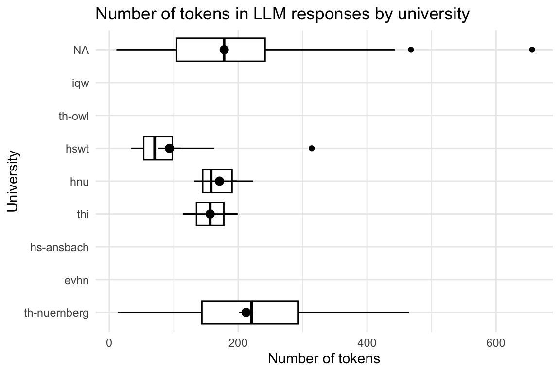
8.9.4 Anzahl der Token nach Kursen
Show the code
| course | Variable | Mean | SD | IQR | Range | Skewness | Kurtosis | n | n_Missing |
|---|---|---|---|---|---|---|---|---|---|
| anis2 | tokens_n | (Inf, -Inf) | 0 | 43 | |||||
| armeufa | tokens_n | (Inf, -Inf) | 0 | 2 | |||||
| bare | tokens_n | 171.00 | 46.87 | 91.00 | (132.00, 223.00) | 1.15 | -1.50 | 3 | 12 |
| bio | tokens_n | (Inf, -Inf) | 0 | 168 | |||||
| biotech | tokens_n | (Inf, -Inf) | 0 | 127 | |||||
| biovete | tokens_n | (Inf, -Inf) | 0 | 244 | |||||
| cta1 | tokens_n | 93.38 | 71.24 | 72.75 | (34.00, 314.00) | 2.27 | 5.78 | 16 | 1101 |
| daba | tokens_n | 173.00 | 0.00 | (173.00, 173.00) | 1 | 197 | |||
| enerbi | tokens_n | (Inf, -Inf) | 0 | 10 | |||||
| epsy | tokens_n | (Inf, -Inf) | 0 | 1 | |||||
| etechde | tokens_n | (Inf, -Inf) | 0 | 3 | |||||
| fodesoa | tokens_n | 256.00 | 0.00 | (256.00, 256.00) | 1 | 324 | |||
| fomesoa | tokens_n | (Inf, -Inf) | 0 | 6 | |||||
| fosaq | tokens_n | (Inf, -Inf) | 0 | 60 | |||||
| gdi | tokens_n | 185.00 | 5.00 | 10.00 | (180.00, 190.00) | 0.00 | -1.50 | 3 | 47 |
| gemwesa | tokens_n | (Inf, -Inf) | 0 | 57 | |||||
| gesoa | tokens_n | 186.41 | 126.56 | 217.00 | (13.00, 450.00) | 0.36 | -1.02 | 64 | 2319 |
| kore | tokens_n | (Inf, -Inf) | 0 | 3 | |||||
| mat11akzg | tokens_n | (Inf, -Inf) | 0 | 2 | |||||
| mibio | tokens_n | (Inf, -Inf) | 0 | 206 | |||||
| mioek | tokens_n | 156.50 | 60.10 | 85.00 | (114.00, 199.00) | 0.00 | -2.00 | 2 | 435 |
| nlp | tokens_n | 356.50 | 153.44 | 217.00 | (248.00, 465.00) | 0.00 | -2.00 | 2 | 65 |
| quame1 | tokens_n | (Inf, -Inf) | 0 | 3 | |||||
| quanch | tokens_n | (Inf, -Inf) | 0 | 34 | |||||
| softa | tokens_n | (Inf, -Inf) | 0 | 4 | |||||
| thesoa | tokens_n | 249.38 | 73.66 | 106.00 | (15.00, 394.00) | -0.87 | 1.23 | 39 | 273 |
| wirkori | tokens_n | (Inf, -Inf) | 0 | 5 | |||||
| wisoa | tokens_n | (Inf, -Inf) | 0 | 33 | |||||
| zemiws | tokens_n | (Inf, -Inf) | 0 | 1 |
Show the code
llm_response_text_date_course_uni |>
  ggboxplot(
    x = "course",
    y = "tokens_n",
    add = "mean_se"
  ) +
  theme_minimal() +
  labs(
    title = "Number of tokens in LLM responses by course",
    x = "Course",
    y = "Number of tokens"
  ) +
  coord_flip()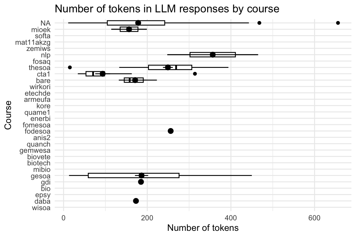
8.9.5 Anzahl vorab existierender Fragen
8.9.5.1 Anzahl verify_option_wrong und verify_option_correct
8.9.5.1.1 idvisit
Show the code
verify_option_summary <- as.data.table(data_separated_filtered)[,
  .(idvisit, value) # keep only needed columns
][
  value %chin% c("verify_option_wrong", "verify_option_correct"), # filter
  .(verify_option = .N), # summarise count
  by = idvisit
]

verify_option_summary <- as_tibble(verify_option_summary)
Show the code
verify_option_summary |>
  gghistogram(x = "verify_option")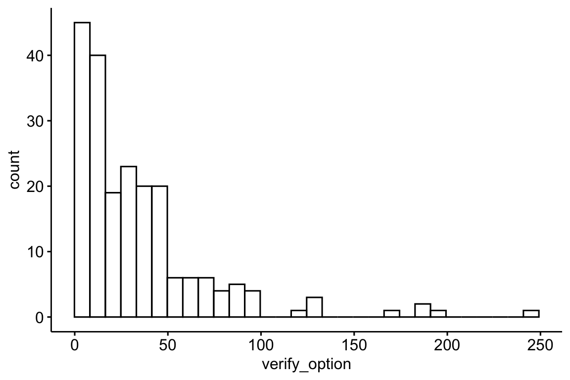
Show the code
verify_option_summary |>
  describe_distribution(verify_option) |>
print_md()| Variable | Mean | SD | IQR | Range | Skewness | Kurtosis | n | n_Missing |
|---|---|---|---|---|---|---|---|---|
| verify_option | 35.24 | 36.76 | 30 | (4.00, 245.00) | 2.64 | 9.11 | 207 | 0 |
8.9.5.1.2 fingerprint unique
Show the code
# verify_option_summary_fingerprint <-
#   data_separated_filtered |>
#   group_by(fingerprint) |>
#   filter(value == "verify_option_wrong" | value == "verify_option_correct") |>
#   summarise(verify_option = n())

setDT(data_separated_filtered) # Ensure your data frame is a data.table

verify_option_summary_fingerprint <- data_separated_filtered[
  # 1. Filtering (i)
  value %in% c("verify_option_wrong", "verify_option_correct"),

  # 2. Summarize (.j) - calculate the count (n)
  .(verify_option = .N),

  # 3. Grouping (by)
  by = .(fingerprint)
]

verify_option_summary_fingerprint <- as_tibble(
  verify_option_summary_fingerprint
)
Show the code
verify_option_summary_fingerprint |>
  gghistogram(x = "verify_option")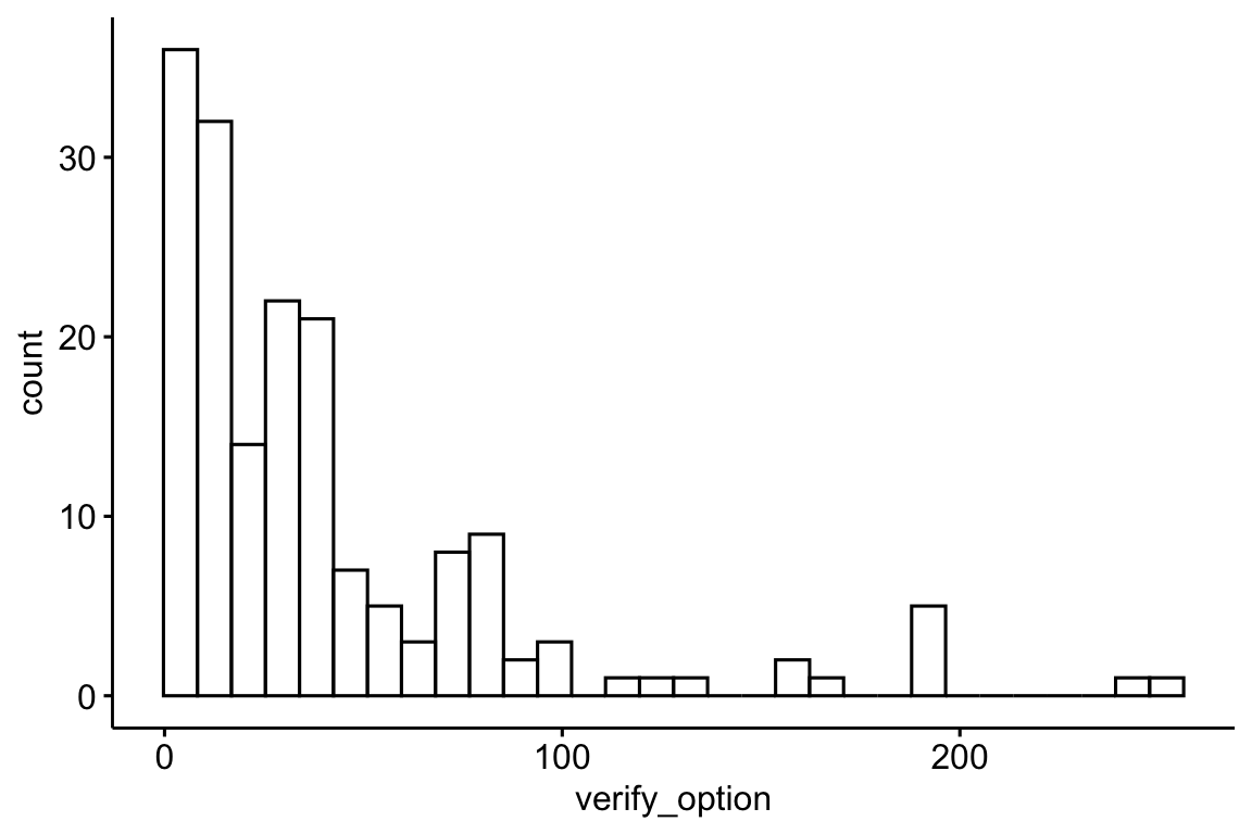
Show the code
verify_option_summary_fingerprint |>
  describe_distribution(verify_option) |>
print_md()| Variable | Mean | SD | IQR | Range | Skewness | Kurtosis | n | n_Missing |
|---|---|---|---|---|---|---|---|---|
| verify_option | 41.68 | 46.81 | 35 | (4.00, 252.00) | 2.35 | 5.94 | 175 | 0 |
8.9.5.2 Anzahl verify_option_wrong verify_option_div_by_4 - geteilt durch 4
Show the code
verify_option_summary <-
  verify_option_summary |>
  mutate(verify_option_div_by_4 = verify_option / 4)

verify_option_summary |>
  gghistogram(x = "verify_option_div_by_4")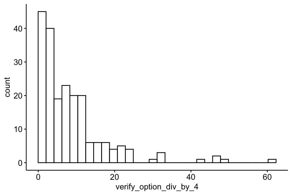
8.9.5.3 Anzahl “Multiple choice answer selected”
Show the code
| n | verify_option | verify_option_div_by_4 |
|---|---|---|
| 1560 | ||
| 6 | 28 | 7.00 |
| 1569 | ||
| 2 | 14 | 3.50 |
| 2021 | ||
| 2 | 21 | 5.25 |
| 2022 | ||
| 10 | 126 | 31.50 |
| 2394 | ||
| 2 | 21 | 5.25 |
| 2718 | ||
| 2 | 7 | 1.75 |
| 2740 | ||
| 2 | 7 | 1.75 |
| 2883 | ||
| 2 | 126 | 31.50 |
| 2902 | ||
| 2 | 126 | 31.50 |
| 2912 | ||
| 2 | 77 | 19.25 |
| 2932 | ||
| 6 | 35 | 8.75 |
| 2950 | ||
| 2 | 56 | 14.00 |
| 2978 | ||
| 14 | 245 | 61.25 |
| 2979 | ||
| 4 | 35 | 8.75 |
| 3103 | ||
| 2 | 14 | 3.50 |
| 3257 | ||
| 2 | 7 | 1.75 |
| 3691 | ||
| 2 | 35 | 8.75 |
| 3700 | ||
| 4 | 84 | 21.00 |
| 3741 | ||
| 2 | 21 | 5.25 |
| 3804 | ||
| 2 | 70 | 17.50 |
Nein, beide Methoden liefern nicht die gleiche Zahl.
8.9.5.4 “Multiple choice answer selected” im Zeitverlauf
Show the code
mc_answers_with_timestamps <-
  mc_answers_with_timestamps |>
  mutate(month_start = floor_date(timestamp, "month")) |>
  ungroup() |>
  arrange(timestamp) |>
  mutate(n_cumulated = cumsum(n)) |>
  mutate(date = as.Date(timestamp))

lim <- c(
  floor_date(min(mc_answers_with_timestamps$date), unit = "year"),
  max(mc_answers_with_timestamps$date)
)

rect_data <- comp_semester_rects(mc_answers_with_timestamps, col_date = "date")

mc_answers_with_timestamps |>
  ggplot(aes(x = date, y = n_cumulated)) +
  scale_x_date(limits = lim, labels = scales::label_date_short()) +
  geom_rect(
    data = rect_data,
    aes(xmin = xmin, xmax = xmax, ymin = ymin, ymax = ymax),
    fill = "grey",
    alpha = 0.2,
    inherit.aes = FALSE # Essential to use the rect_data columns
  ) +
  geom_point() +
  geom_line()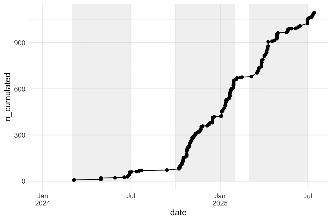
8.9.5.5 Anzahl generate_questionaire
Show the code
# generate_questionaire_summary <-
#   data_separated_filtered |>
#   group_by(idvisit) |>
#   filter(value == "generate_questionaire") |>
#   summarise(generate_questionaire = n())

setDT(data_separated_filtered) # Convert the data.frame to a data.table in place

generate_questionaire_summary <- data_separated_filtered[
  # 1. Filtering (i)
  value == "generate_questionaire",

  # 2. Summarize (.j) - calculate the count (.N) and rename it
  .(generate_questionaire = .N),

  # 3. Grouping (by)
  by = .(idvisit)
]
Show the code
generate_questionaire_summary |>
  describe_distribution(generate_questionaire) |>
print_md()| Variable | Mean | SD | IQR | Range | Skewness | Kurtosis | n | n_Missing |
|---|---|---|---|---|---|---|---|---|
| generate_questionaire | 3.11 | 5.93 | 2 | (1.00, 66.00) | 5.89 | 46.07 | 367 | 0 |
8.9.5.6 Anzahl vorab existierender Fragen
Show the code
setDT(generate_questionaire_summary)
setDT(verify_option_summary)

# 1. Full Join (Merge)
# Use the 'merge' function with all.x=TRUE and all.y=TRUE for a full join
# Assumes the join column is 'idvisit' as used in your previous examples
prior_existing_questions_summary <- merge(
  generate_questionaire_summary,
  verify_option_summary,
  by = "idvisit",
  all = TRUE
)

# 2. Mutate (Calculation)
# Use .j to create the new column
prior_existing_questions_summary[,
  prior_existing_questions_n := verify_option - generate_questionaire
]

# prior_existing_questions_summary <-
#   generate_questionaire_summary |>
#   full_join(verify_option_summary) |>
#   mutate(prior_existing_questions_n = verify_option - generate_questionaire)
Show the code
prior_existing_questions_summary |>
  # drop_na() |>
  gghistogram(x = "prior_existing_questions_n")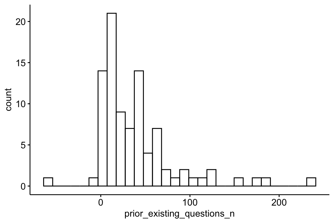
Show the code
prior_existing_questions_summary |>
  describe_distribution(prior_existing_questions_n) |>
print_md()| Variable | Mean | SD | IQR | Range | Skewness | Kurtosis | n | n_Missing |
|---|---|---|---|---|---|---|---|---|
| prior_existing_questions_n | 38.87 | 44.57 | 39 | (-59.00, 236.00) | 1.98 | 5.40 | 91 | 392 |
8.10 Input zum LLM: message_to_llm - Tokens und Tokenlänge
Show the code
prompt_length |>
  head()
Show the code
prompt_length |>
  describe_distribution(token_length)
Show the code
prompt_length |>
  ggplot(aes(x = token_length)) +
  geom_histogram(binwidth = 10) +
  labs(
    title = "Length of prompts sent to the LLM",
    x = "Prompt length (in tokens)",
    y = "Number of prompts"
  ) +
  theme_minimal()