3 Zeitraum

3.1 Setup

Show the code

library(tidyverse)
library(lubridate)
library(gt)
library(visdat)
library(data.table)
#library(collapse)
library(targets)
library(easystats)
library(scales)

Show the code

source("_common.r")

Show the code

tar_load(c(
  course_and_uni_per_visit,
  n_action,
  n_action_w_date,
  time_since_last_visit,
  time_visit_wday,
  n_action_fingerprint,
  time_visit_wday_fingerprint,
  data_separated_filtered,
  n_action_lt_500,
  n_action_lt_500_fingerprint
))

3.2 Beginn/Ende der Daten

Show the code

n_action_w_date |>
  head(30)

Show the code

min_max_time <-
  n_action_w_date |>
  summarise(
    time_min = min(date_time_start, na.rm = T),
    time_max = max(date_time_start, na.rm = T)
  )

min_max_time |>
  gt()

time_min	time_max
2022-12-05 15:33:45	2025-07-14 23:40:45

Wichtig

Erster Visit im Datensatz: 2022-12-05 15:33:45.

Letzter Visit im Datensatz: 2025-07-14 23:40:45.

Diese Statistik wurde auf Basis des Datenobjekts data_separated_filtered berechnet, vgl. das Target dieses Objekts in der Pipeline.

3.3 Days since last visit

3.3.1 Insgesamt

3.3.1.1 idvisit

Show the code

time_visit_wday |>
  head(30)

Show the code

time_since_last_visit <-
  time_since_last_visit |>
  mutate(dayssincelastvisit = as.numeric(dayssincelastvisit)) |>
  distinct(idvisit, .keep_all = TRUE)

time_since_last_visit |>
  datawizard::describe_distribution(dayssincelastvisit) |>
  knitr::kable(digits = 2)

Variable	Mean	SD	IQR	Min	Max	Skewness	Kurtosis	n	n_Missing
dayssincelastvisit	6.89	15.75	0	1	87	2.98	8.26	14207	0

Show the code

time_since_last_visit |>
  ggplot(aes(x = dayssincelastvisit)) +
  geom_density() +
  labs(
    title = "If visitor return, they return mostly not later than a few days."
  )

Wichtig

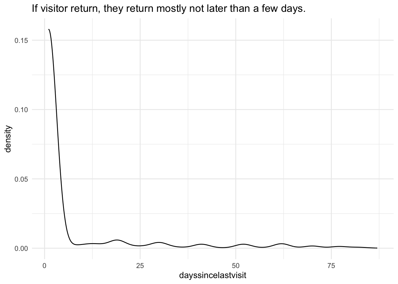
Die Nutzer nutzen die Seite in Abständen von wenigen Tagen?

3.3.1.2 fingerprint unique

Show the code

time_visit_wday_fingerprint |> head()

Show the code

time_since_last_visit_fingerprint <-
  time_since_last_visit |>
  mutate(dayssincelastvisit = as.numeric(dayssincelastvisit)) |>
  distinct(fingerprint, .keep_all = TRUE)

time_since_last_visit |>
  datawizard::describe_distribution(dayssincelastvisit) |>
  knitr::kable(digits = 2)

Variable	Mean	SD	IQR	Min	Max	Skewness	Kurtosis	n	n_Missing
dayssincelastvisit	6.89	15.75	0	1	87	2.98	8.26	14207	0

Show the code

time_since_last_visit |>
  ggplot(aes(x = dayssincelastvisit)) +
  geom_density() +
  labs(
    title = "If visitor return, they return mostly not later than a few days."
  )

3.3.2 Nach Lehrveranstaltungen

Show the code

time_since_last_visit_per_course <-
  time_since_last_visit |>
  left_join(course_and_uni_per_visit) |>
  drop_na()

Show the code

time_since_last_visit_per_course_summary <-
  time_since_last_visit_per_course |>
  group_by(course) |>
  summarise(
    dayssincelastvisit_mean = mean(dayssincelastvisit),
    dayssincelastvisit_sd = sd(dayssincelastvisit),
    dayssincelastvisit_n = n()
  ) |>
  mutate(
    dayssincelastvisit_n_log = log(dayssincelastvisit_n, base = 10) + 0.001
  )

Show the code

time_since_last_visit_per_course_summary

Show the code

time_since_last_visit_per_course_summary |>
  ggplot(aes(
    y = reorder(course, dayssincelastvisit_mean),
    x = dayssincelastvisit_mean
  )) +
  geom_errorbar(aes(
    xmin = dayssincelastvisit_mean - dayssincelastvisit_sd,
    xmax = dayssincelastvisit_mean + dayssincelastvisit_sd
  )) +
  geom_point(aes(alpha = log(dayssincelastvisit_n)), show.legend = FALSE) +
  labs(
    x = "Days since last visit (mean±sd)",
    y = "course",
    title = "In some courses, users use HaNS frequently.",
    caption = "Grey saturation of the mean dots refers to the log10 of the sample size (N)"
  ) +
  geom_text(
    aes(label = round(dayssincelastvisit_n)),
    x = Inf,
    hjust = 1.2,
    size = 2
  ) +
  annotate(
    x = Inf,
    y = Inf,
    label = "N",
    geom = "label",
    hjust = 1,
    vjust = 1
  ) +
  scale_y_discrete(expand = expansion(mult = 0.1)) +
  theme_minimal()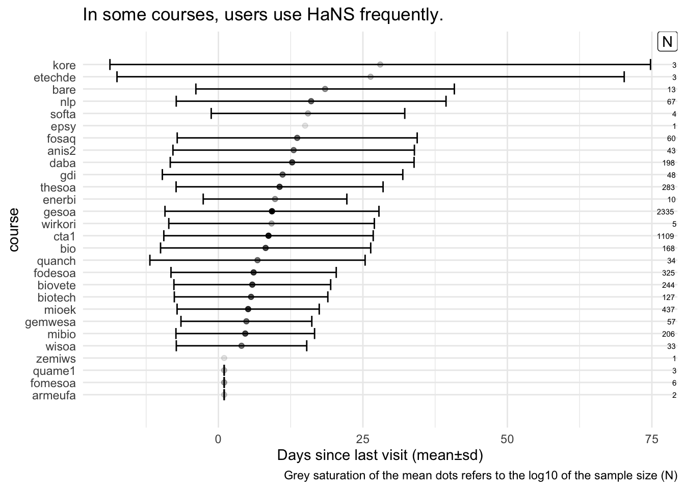

3.4 Visits im Zeitverlauf

Wie viele Visits (von Hans) gab es?

3.4.1 Visits im Zeitverlauf - üro Monat

3.4.1.1 idivisit

Show the code

time_visit_wday_summary <-
  time_visit_wday |>
  ungroup() |>
  mutate(month_start = floor_date(date_time, "month")) |>
  mutate(
    month_name = lubridate::month(date_time, label = TRUE, abbr = FALSE),
    month_num = lubridate::month(date_time, label = FALSE),
    year_num = lubridate::year(date_time)
  )

Show the code

time_visit_wday_summary |>
  group_by(year_num, month_num) |>
  summarise(n = n()) |>
  gt()

month_num	n
2022
12	329
2023
1	455
2	561
3	149
4	253
5	391
6	292
7	441
8	26
9	39
10	614
11	660
12	519
2024
1	783
2	85
3	138
4	329
5	413
6	593
7	743
8	16
9	23
10	731
11	918
12	765
2025
1	959
2	155
3	507
4	1011
5	557
6	321
7	430
NA
NA	1

Show the code

time_visit_wday_summary |>
  group_by(year_num, month_start) |>
  summarise(n = n()) |>
  ggplot(aes(x = month_start, y = n)) +
  geom_line(group = 1, color = "grey60") +
  geom_point() +
  labs(
    title = "The number of visits reflect the teaching periods of the semesters.",
    x = "month/year"
  ) +
  
  # --- Highlight March–July (approx 1 Mar to 31 Jul) ---
  annotate(
    "rect",
    xmin = as.Date("2023-03-01"),
    xmax = as.Date("2023-07-31"),
    ymin = -Inf,
    ymax = Inf,
    alpha = 0.2,
    fill = "skyblue"
  ) +

  annotate(
    "rect",
    xmin = as.Date("2024-03-01"),
    xmax = as.Date("2024-07-31"),
    ymin = -Inf,
    ymax = Inf,
    alpha = 0.2,
    fill = "skyblue"
  ) +
  annotate(
    "rect",
    xmin = as.Date("2025-03-01"),
    xmax = as.Date("2025-07-31"),
    ymin = -Inf,
    ymax = Inf,
    alpha = 0.2,
    fill = "skyblue"
  ) +

  # --- Highlight October–February (semester break or 2nd term) ---
  annotate(
    "rect",
    xmin = as.Date("2023-10-01"),
    xmax = as.Date("2024-02-28"),
    ymin = -Inf,
    ymax = Inf,
    alpha = 0.2,
    fill = "orange"
  ) +
  # annotate("rect",
  #          xmin = as.Date("2024-10-01"), xmax = as.Date("2024-02-28"),
  #          ymin = -Inf, ymax = Inf, alpha = 0.2, fill = "orange") +
  annotate(
    "rect",
    xmin = as.Date("2024-10-01"),
    xmax = as.Date("2025-02-28"),
    ymin = -Inf,
    ymax = Inf,
    alpha = 0.2,
    fill = "orange"
  ) +

  # --- Your data lines ---
  geom_line(group = 1, color = "grey60") +
  geom_point() +
  labs(
    title = "The number of visits reflect the teaching periods of the semesters.",
    x = "month/year"
  ) +
  theme_minimal() +
  geom_smooth(method = "loess", se = FALSE, color = "blue")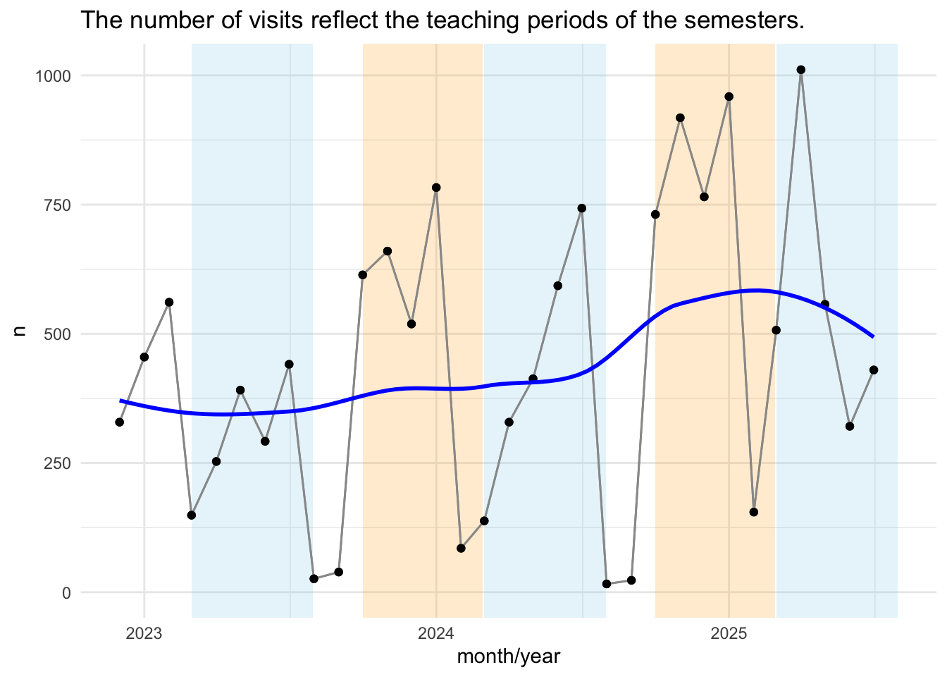

3.4.1.2 fingerprint

Show the code

time_visit_wday_summary_fingerprint <-
  time_visit_wday_fingerprint |>
  ungroup() |>
  mutate(month_start = floor_date(date_time, "month")) |>
  mutate(
    month_name = lubridate::month(date_time, label = TRUE, abbr = FALSE),
    month_num = lubridate::month(date_time),
    year_num = lubridate::year(date_time)
  )

Show the code

time_visit_wday_summary_fingerprint |>
  group_by(year_num, month_num) |>
  summarise(n = n()) |>
  gt()

month_num	n
2022
12	235
2023
1	248
2	303
3	99
4	160
5	226
6	195
7	227
8	17
9	23
10	402
11	412
12	325
2024
1	445
2	50
3	94
4	179
5	204
6	274
7	214
8	10
9	16
10	365
11	417
12	317
2025
1	347
2	74
3	217
4	424
5	273
6	171
7	196
NA
NA	1

Show the code

time_visit_wday_summary_fingerprint |>
  group_by(year_num, month_start) |>
  summarise(n = n()) |>
  ggplot(aes(x = month_start, y = n)) +
  geom_line(group = 1, color = "grey60") +
  geom_point() +
  labs(
    title = "The number of visits reflect the teaching periods of the semesters.",
    x = "month/year"
  ) +

  # --- Highlight March–July (approx 1 Mar to 31 Jul) ---
  annotate(
    "rect",
    xmin = as.Date("2023-03-01"),
    xmax = as.Date("2023-07-31"),
    ymin = -Inf,
    ymax = Inf,
    alpha = 0.2,
    fill = "skyblue"
  ) +

  annotate(
    "rect",
    xmin = as.Date("2024-03-01"),
    xmax = as.Date("2024-07-31"),
    ymin = -Inf,
    ymax = Inf,
    alpha = 0.2,
    fill = "skyblue"
  ) +
  annotate(
    "rect",
    xmin = as.Date("2025-03-01"),
    xmax = as.Date("2025-07-31"),
    ymin = -Inf,
    ymax = Inf,
    alpha = 0.2,
    fill = "skyblue"
  ) +

  # --- Highlight October–February (semester break or 2nd term) ---
  annotate(
    "rect",
    xmin = as.Date("2023-10-01"),
    xmax = as.Date("2024-02-28"),
    ymin = -Inf,
    ymax = Inf,
    alpha = 0.2,
    fill = "orange"
  ) +
  # annotate("rect",
  #          xmin = as.Date("2024-10-01"), xmax = as.Date("2024-02-28"),
  #          ymin = -Inf, ymax = Inf, alpha = 0.2, fill = "orange") +
  annotate(
    "rect",
    xmin = as.Date("2024-10-01"),
    xmax = as.Date("2025-02-28"),
    ymin = -Inf,
    ymax = Inf,
    alpha = 0.2,
    fill = "orange"
  ) +

  # --- Your data lines ---
  geom_line(group = 1, color = "grey60") +
  geom_point() +
  labs(
    title = "The number of visits reflect the teaching periods of the semesters.",
    x = "month/year"
  ) +
  theme_minimal() +
  geom_smooth(method = "loess", se = FALSE, color = "blue")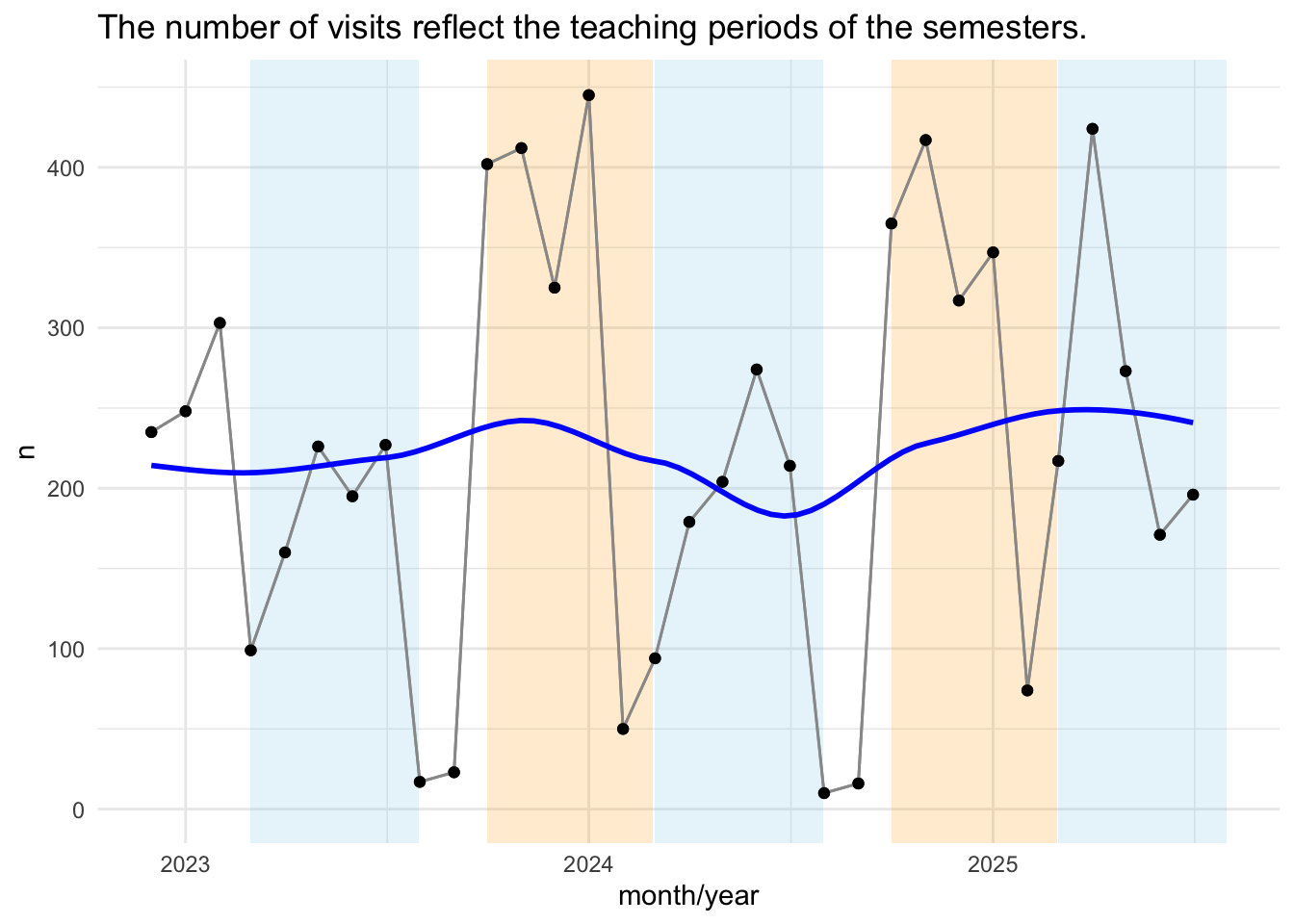

Show the code

library(ggplot2)
library(dplyr)
library(lubridate)

time_visit_wday_summary_fingerprint |>
  group_by(year_num, month_start) |>
  summarise(n = n()) |>
  ggplot(aes(x = month_start, y = n)) +

  # --- Highlight March–July (approx 1 Mar to 31 Jul) ---
  annotate(
    "rect",
    xmin = as.Date("2023-03-01"),
    xmax = as.Date("2023-07-31"),
    ymin = -Inf,
    ymax = Inf,
    alpha = 0.2,
    fill = "skyblue"
  ) +

  annotate(
    "rect",
    xmin = as.Date("2024-03-01"),
    xmax = as.Date("2024-07-31"),
    ymin = -Inf,
    ymax = Inf,
    alpha = 0.2,
    fill = "skyblue"
  ) +
  annotate(
    "rect",
    xmin = as.Date("2025-03-01"),
    xmax = as.Date("2025-07-31"),
    ymin = -Inf,
    ymax = Inf,
    alpha = 0.2,
    fill = "skyblue"
  ) +

  # --- Highlight October–February (semester break or 2nd term) ---
  annotate(
    "rect",
    xmin = as.Date("2023-10-01"),
    xmax = as.Date("2024-02-28"),
    ymin = -Inf,
    ymax = Inf,
    alpha = 0.2,
    fill = "orange"
  ) +
  # annotate("rect",
  #          xmin = as.Date("2024-10-01"), xmax = as.Date("2024-02-28"),
  #          ymin = -Inf, ymax = Inf, alpha = 0.2, fill = "orange") +
  annotate(
    "rect",
    xmin = as.Date("2024-10-01"),
    xmax = as.Date("2025-02-28"),
    ymin = -Inf,
    ymax = Inf,
    alpha = 0.2,
    fill = "orange"
  ) +

  # --- Your data lines ---
  geom_line(group = 1, color = "grey60") +
  geom_point() +
  labs(
    title = "The number of visits reflect the teaching periods of the semesters.",
    x = "month/year"
  ) +
  theme_minimal() +
  geom_smooth(method = "loess", se = FALSE, color = "blue")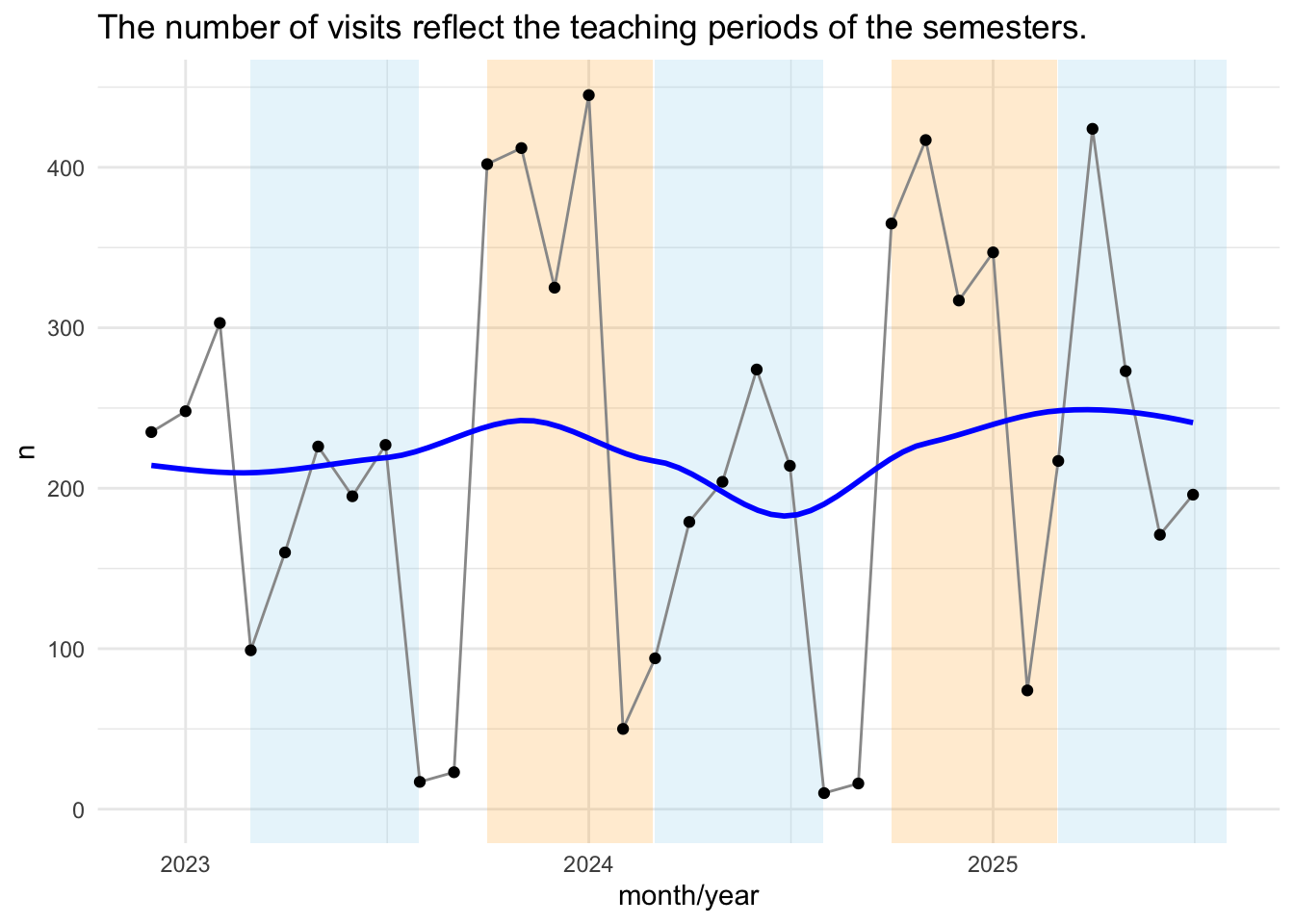

3.4.1.3 fingerprint unique

Show the code

time_visit_wday_summary_fingerprint_unique <-
  time_visit_wday_fingerprint |>
  ungroup() |>
  distinct(fingerprint, .keep_all = TRUE) |>
  mutate(month_start = floor_date(date_time, "month")) |>
  mutate(
    month_name = lubridate::month(date_time, label = TRUE, abbr = FALSE),
    month_num = lubridate::month(date_time),
    year_num = lubridate::year(date_time)
  )

Show the code

time_visit_wday_summary_fingerprint_unique |>
  group_by(year_num, month_num) |>
  summarise(n = n()) |>
  gt()

month_num	n
2022
12	235
2023
1	248
2	303
3	99
4	160
5	226
6	195
7	227
8	17
9	23
10	402
11	412
12	325
2024
1	445
2	50
3	94
4	179
5	204
6	274
7	214
8	10
9	16
10	365
11	417
12	317
2025
1	347
2	74
3	217
4	424
5	273
6	171
7	196
NA
NA	1

Show the code

time_visit_wday_summary_fingerprint_unique |>
  group_by(year_num, month_start) |>
  summarise(n = n()) |>
  ggplot(aes(x = month_start, y = n)) +
  geom_line(group = 1, color = "grey60") +
  geom_point() +
  labs(
    title = "The number of visits reflect the teaching periods of the semesters.",
    x = "month/year"
  ) +
    
  # --- Highlight March–July (approx 1 Mar to 31 Jul) ---
  annotate(
    "rect",
    xmin = as.Date("2023-03-01"),
    xmax = as.Date("2023-07-31"),
    ymin = -Inf,
    ymax = Inf,
    alpha = 0.2,
    fill = "skyblue"
  ) +

  annotate(
    "rect",
    xmin = as.Date("2024-03-01"),
    xmax = as.Date("2024-07-31"),
    ymin = -Inf,
    ymax = Inf,
    alpha = 0.2,
    fill = "skyblue"
  ) +
  annotate(
    "rect",
    xmin = as.Date("2025-03-01"),
    xmax = as.Date("2025-07-31"),
    ymin = -Inf,
    ymax = Inf,
    alpha = 0.2,
    fill = "skyblue"
  ) +

  # --- Highlight October–February (semester break or 2nd term) ---
  annotate(
    "rect",
    xmin = as.Date("2023-10-01"),
    xmax = as.Date("2024-02-28"),
    ymin = -Inf,
    ymax = Inf,
    alpha = 0.2,
    fill = "orange"
  ) +
  # annotate("rect",
  #          xmin = as.Date("2024-10-01"), xmax = as.Date("2024-02-28"),
  #          ymin = -Inf, ymax = Inf, alpha = 0.2, fill = "orange") +
  annotate(
    "rect",
    xmin = as.Date("2024-10-01"),
    xmax = as.Date("2025-02-28"),
    ymin = -Inf,
    ymax = Inf,
    alpha = 0.2,
    fill = "orange"
  )   +
  geom_smooth(method = "loess", se = FALSE, color = "blue")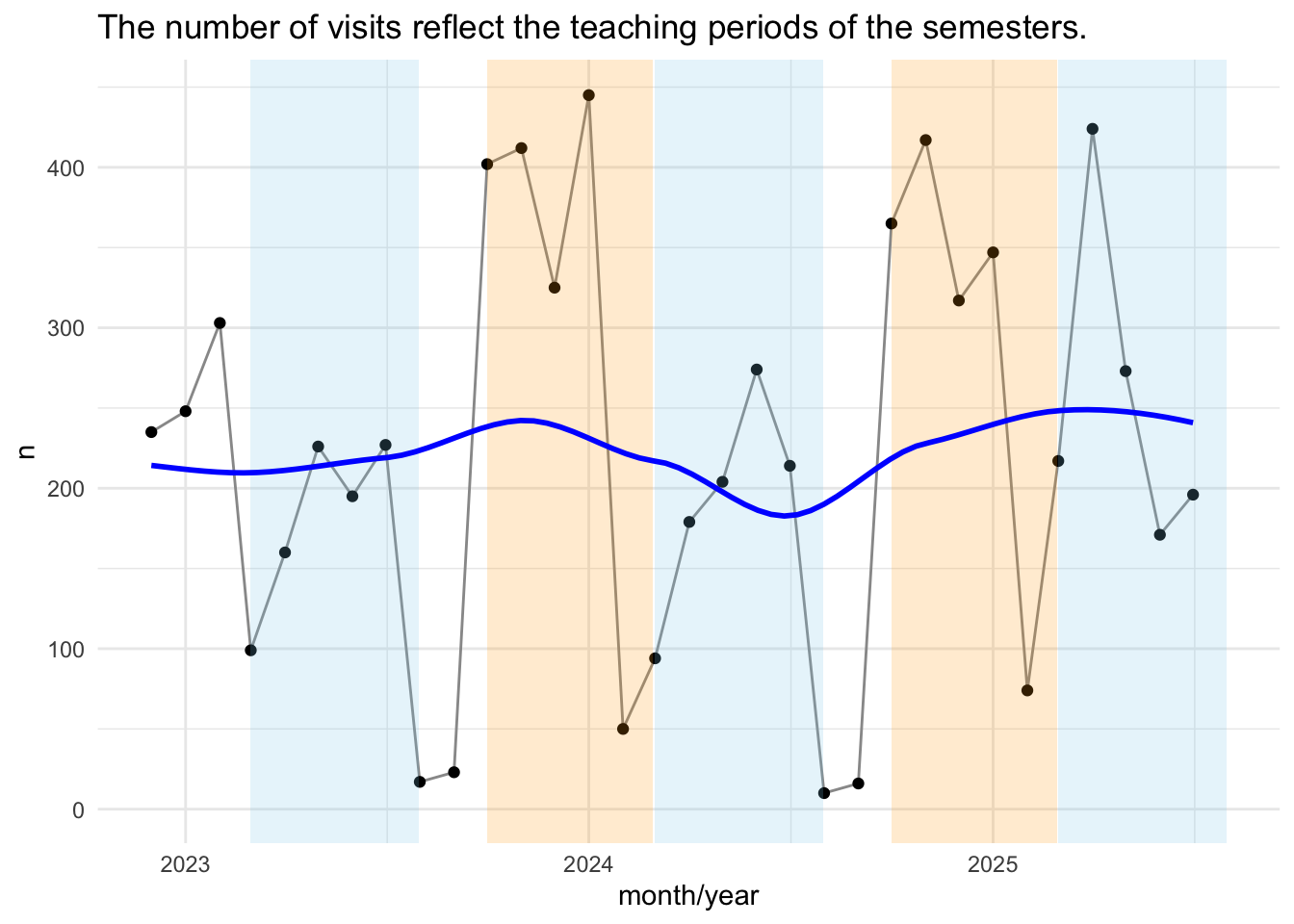

3.4.2 Visits im Zeitverlauf - pro Woche

Show the code

time_visit_wday_summary_week <-
  time_visit_wday |>
  ungroup() |>
  mutate(week_start = floor_date(date_time, "week")) |>
  mutate(week_num = week(date_time), year_num = year(date_time))

Show the code

time_visit_wday_summary_week_summarized <-
  time_visit_wday_summary_week |>
  group_by(year_num, week_num) |>
  summarise(n = n())

time_visit_wday_summary_week_summarized

Show the code

time_visit_wday_summary_week_summarized_dateformat <-
  time_visit_wday_summary_week |>
  group_by(week_start) |>
  summarise(n = n())

Show the code

time_visit_wday_summary_week_summarized_dateformat |>
  ggplot(aes(x = week_start, y = n)) +
  geom_line(group = 1, color = "grey60") +
  geom_point() +
  geom_smooth(method = "gam", se = FALSE, color = "blue") +
  labs(
    title = "The number of visits is increasing and reflects the teaching periods of the semesters.",
    x = "week number/year"
  ) +

  # --- Highlight March–July (approx 1 Mar to 31 Jul) ---
  annotate(
    "rect",
    xmin = as.Date("2023-03-01"),
    xmax = as.Date("2023-07-31"),
    ymin = -Inf,
    ymax = Inf,
    alpha = 0.2,
    fill = "skyblue"
  ) +

  annotate(
    "rect",
    xmin = as.Date("2024-03-01"),
    xmax = as.Date("2024-07-31"),
    ymin = -Inf,
    ymax = Inf,
    alpha = 0.2,
    fill = "skyblue"
  ) +
  annotate(
    "rect",
    xmin = as.Date("2025-03-01"),
    xmax = as.Date("2025-07-31"),
    ymin = -Inf,
    ymax = Inf,
    alpha = 0.2,
    fill = "skyblue"
  ) +

  # --- Highlight October–February (semester break or 2nd term) ---
  annotate(
    "rect",
    xmin = as.Date("2023-10-01"),
    xmax = as.Date("2024-02-28"),
    ymin = -Inf,
    ymax = Inf,
    alpha = 0.2,
    fill = "orange"
  ) +
  # annotate("rect",
  #          xmin = as.Date("2024-10-01"), xmax = as.Date("2024-02-28"),
  #          ymin = -Inf, ymax = Inf, alpha = 0.2, fill = "orange") +
  annotate(
    "rect",
    xmin = as.Date("2024-10-01"),
    xmax = as.Date("2025-02-28"),
    ymin = -Inf,
    ymax = Inf,
    alpha = 0.2,
    fill = "orange"
  )   +
  geom_smooth(method = "loess", se = FALSE, color = "blue")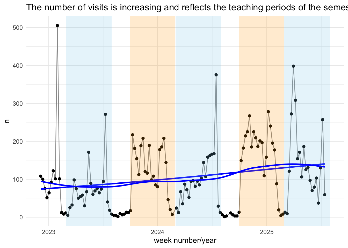

Wichtig

The number of visits has increased over time.

3.4.3 Akkumulierte Seitenaufrufe im Zeitverlauf

3.4.3.1 Monat - idvisit

Show the code

time_visit_wday_summary |>
  group_by(year_num, month_start) |>
  summarise(n = n()) |>
  ungroup() |>
  mutate(n_cumsum = cumsum(n)) |>
  ggplot(aes(x = month_start, y = n_cumsum)) +
  geom_line(group = 1, color = "grey60") +
  geom_point() +
  theme_minimal() +
  geom_smooth(method = "lm") +
  labs(title = "Visits have increased linearly over time.", x = "month/year") +
  annotate(
    "rect",
    xmin = as.Date("2023-03-01"),
    xmax = as.Date("2023-07-31"),
    ymin = -Inf,
    ymax = Inf,
    alpha = 0.2,
    fill = "skyblue"
  ) +

  annotate(
    "rect",
    xmin = as.Date("2024-03-01"),
    xmax = as.Date("2024-07-31"),
    ymin = -Inf,
    ymax = Inf,
    alpha = 0.2,
    fill = "skyblue"
  ) +
  annotate(
    "rect",
    xmin = as.Date("2025-03-01"),
    xmax = as.Date("2025-07-31"),
    ymin = -Inf,
    ymax = Inf,
    alpha = 0.2,
    fill = "skyblue"
  ) +

  # --- Highlight October–February (semester break or 2nd term) ---
  annotate(
    "rect",
    xmin = as.Date("2023-10-01"),
    xmax = as.Date("2024-02-28"),
    ymin = -Inf,
    ymax = Inf,
    alpha = 0.2,
    fill = "orange"
  ) +
  # annotate("rect",
  #          xmin = as.Date("2024-10-01"), xmax = as.Date("2024-02-28"),
  #          ymin = -Inf, ymax = Inf, alpha = 0.2, fill = "orange") +
  annotate(
    "rect",
    xmin = as.Date("2024-10-01"),
    xmax = as.Date("2025-02-28"),
    ymin = -Inf,
    ymax = Inf,
    alpha = 0.2,
    fill = "orange"
   ) +
  geom_smooth(method = "loess", se = FALSE, color = "blue")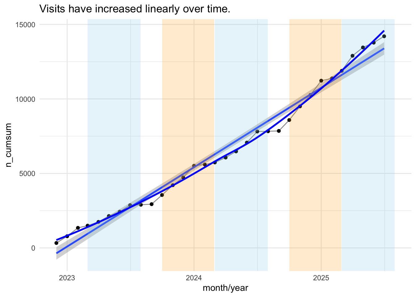

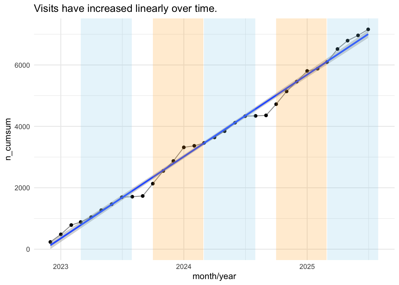
3.4.3.2 Monat - fingerprint

Show the code

time_visit_wday_summary_fingerprint |>
  group_by(year_num, month_start) |>
  summarise(n = n()) |>
  ungroup() |>
  mutate(n_cumsum = cumsum(n)) |>
  ggplot(aes(x = month_start, y = n_cumsum)) +
  geom_line(group = 1, color = "grey60") +
  geom_point() +
  theme_minimal() +
  geom_smooth(method = "lm") +
  labs(title = "Visits have increased linearly over time.", x = "month/year") +
  labs(title = "Visits have increased linearly over time.", x = "month/year") +
  annotate(
    "rect",
    xmin = as.Date("2023-03-01"),
    xmax = as.Date("2023-07-31"),
    ymin = -Inf,
    ymax = Inf,
    alpha = 0.2,
    fill = "skyblue"
  ) +

  annotate(
    "rect",
    xmin = as.Date("2024-03-01"),
    xmax = as.Date("2024-07-31"),
    ymin = -Inf,
    ymax = Inf,
    alpha = 0.2,
    fill = "skyblue"
  ) +
  annotate(
    "rect",
    xmin = as.Date("2025-03-01"),
    xmax = as.Date("2025-07-31"),
    ymin = -Inf,
    ymax = Inf,
    alpha = 0.2,
    fill = "skyblue"
  ) +

  # --- Highlight October–February (semester break or 2nd term) ---
  annotate(
    "rect",
    xmin = as.Date("2023-10-01"),
    xmax = as.Date("2024-02-28"),
    ymin = -Inf,
    ymax = Inf,
    alpha = 0.2,
    fill = "orange"
  ) +
  # annotate("rect",
  #          xmin = as.Date("2024-10-01"), xmax = as.Date("2024-02-28"),
  #          ymin = -Inf, ymax = Inf, alpha = 0.2, fill = "orange") +
  annotate(
    "rect",
    xmin = as.Date("2024-10-01"),
    xmax = as.Date("2025-02-28"),
    ymin = -Inf,
    ymax = Inf,
    alpha = 0.2,
    fill = "orange"
  )

3.4.3.3 Monat - fingerprint unique

Show the code

time_visit_wday_summary_fingerprint_unique |>
  group_by(year_num, month_start) |>
  summarise(n = n()) |>
  ungroup() |>
  mutate(n_cumsum = cumsum(n)) |>
  ggplot(aes(x = month_start, y = n_cumsum)) +
  geom_line(group = 1, color = "grey60") +
  geom_point() +
  theme_minimal() +
  geom_smooth(method = "lm") +
  labs(title = "Visits have increased linearly over time.", x = "month/year") +
  labs(title = "Visits have increased linearly over time.", x = "month/year") +
  annotate(
    "rect",
    xmin = as.Date("2023-03-01"),
    xmax = as.Date("2023-07-31"),
    ymin = -Inf,
    ymax = Inf,
    alpha = 0.2,
    fill = "skyblue"
  ) +

  annotate(
    "rect",
    xmin = as.Date("2024-03-01"),
    xmax = as.Date("2024-07-31"),
    ymin = -Inf,
    ymax = Inf,
    alpha = 0.2,
    fill = "skyblue"
  ) +
  annotate(
    "rect",
    xmin = as.Date("2025-03-01"),
    xmax = as.Date("2025-07-31"),
    ymin = -Inf,
    ymax = Inf,
    alpha = 0.2,
    fill = "skyblue"
  ) +

  # --- Highlight October–February (semester break or 2nd term) ---
  annotate(
    "rect",
    xmin = as.Date("2023-10-01"),
    xmax = as.Date("2024-02-28"),
    ymin = -Inf,
    ymax = Inf,
    alpha = 0.2,
    fill = "orange"
  ) +
  # annotate("rect",
  #          xmin = as.Date("2024-10-01"), xmax = as.Date("2024-02-28"),
  #          ymin = -Inf, ymax = Inf, alpha = 0.2, fill = "orange") +
  annotate(
    "rect",
    xmin = as.Date("2024-10-01"),
    xmax = as.Date("2025-02-28"),
    ymin = -Inf,
    ymax = Inf,
    alpha = 0.2,
    fill = "orange"
  ) +
  geom_smooth(method = "loess", se = FALSE, color = "blue")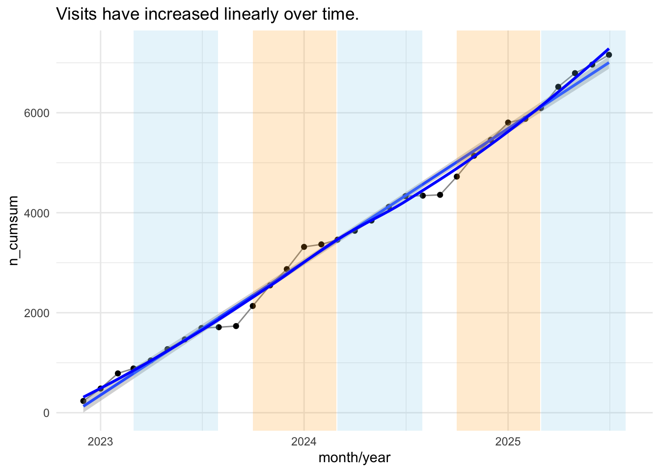

3.4.3.4 Woche

Show the code

time_visit_wday_summary_week |>
  group_by(year_num, week_start) |>
  summarise(n = n()) |>
  ungroup() |>
  mutate(n_cumsum = cumsum(n)) |>
  ggplot(aes(x = week_start, y = n_cumsum)) +
  geom_line(group = 1, color = "grey60") +
  geom_point() +
  theme_minimal() +
  geom_smooth(method = "lm") +
  labs(
    title = "Visits have increased approx. linearly over time.",
    x = "week/year"
  ) +
  labs(title = "Visits have increased linearly over time.", x = "month/year") +
  annotate(
    "rect",
    xmin = as.Date("2023-03-01"),
    xmax = as.Date("2023-07-31"),
    ymin = -Inf,
    ymax = Inf,
    alpha = 0.2,
    fill = "skyblue"
  ) +

  annotate(
    "rect",
    xmin = as.Date("2024-03-01"),
    xmax = as.Date("2024-07-31"),
    ymin = -Inf,
    ymax = Inf,
    alpha = 0.2,
    fill = "skyblue"
  ) +
  annotate(
    "rect",
    xmin = as.Date("2025-03-01"),
    xmax = as.Date("2025-07-31"),
    ymin = -Inf,
    ymax = Inf,
    alpha = 0.2,
    fill = "skyblue"
  ) +

  # --- Highlight October–February (semester break or 2nd term) ---
  annotate(
    "rect",
    xmin = as.Date("2023-10-01"),
    xmax = as.Date("2024-02-28"),
    ymin = -Inf,
    ymax = Inf,
    alpha = 0.2,
    fill = "orange"
  ) +
  # annotate("rect",
  #          xmin = as.Date("2024-10-01"), xmax = as.Date("2024-02-28"),
  #          ymin = -Inf, ymax = Inf, alpha = 0.2, fill = "orange") +
  annotate(
    "rect",
    xmin = as.Date("2024-10-01"),
    xmax = as.Date("2025-02-28"),
    ymin = -Inf,
    ymax = Inf,
    alpha = 0.2,
    fill = "orange"
  ) +
  geom_smooth(method = "loess", se = FALSE, color = "blue")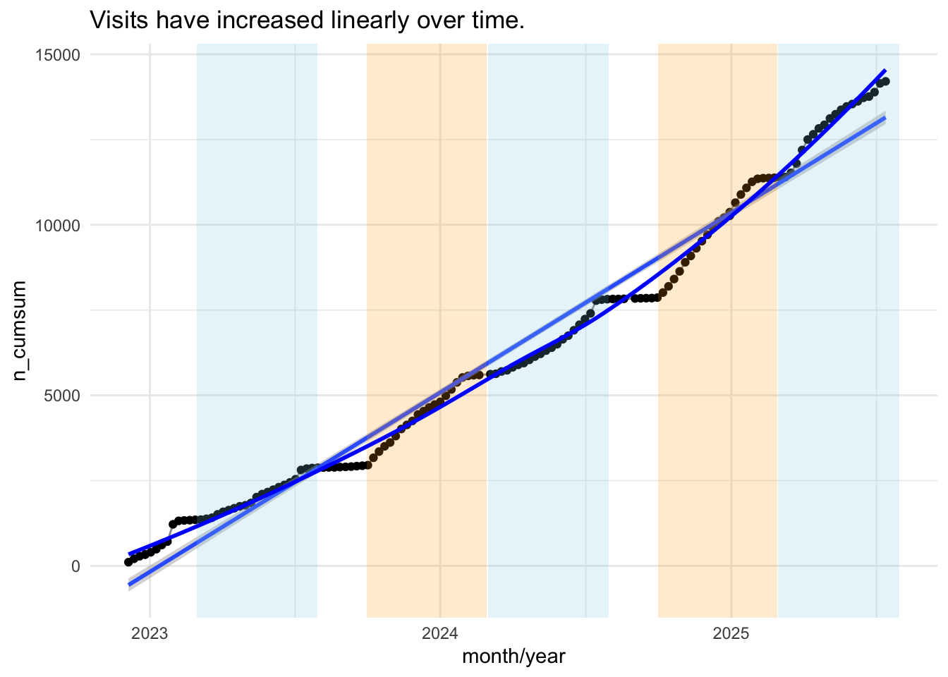

3.5 Statistiken

Die folgenden Statistiken beruhen auf dem Datensatz data_separated_filtered:

3.5.1 idivisit

Show the code

glimpse(data_separated_filtered)

Rows: 4,477,584
Columns: 5
$ nr          <int> 0, 0, 1, 1, 1, 1, 2, 2, 3, 3, 3, 3, 4, 4, 4, 4, 5, 5, 5, 5…
$ type        <fct> subtitle, timestamp, eventcategory, eventaction, timestamp…
$ value       <fct> "https://hans.th-nuernberg.de/", "2023-03-23 18:37:56", "c…
$ idvisit     <int> 1, 1, 1, 1, 1, 1, 1, 1, 1, 1, 1, 1, 1, 1, 1, 1, 1, 1, 1, 1…
$ fingerprint <fct> aa8a78771b4f21ff, aa8a78771b4f21ff, aa8a78771b4f21ff, aa8a…

nr fasst die Nummer der Aktion innerhalb eines bestimmten Visits.

3.5.2 fingerprint unique

Show the code

data_separated_filtered |>
  distinct(fingerprint, .keep_all = TRUE) |>
  glimpse()

Rows: 7,160
Columns: 5
$ nr          <int> 0, 0, 0, 0, 0, 0, 0, 0, 0, 0, 0, 0, 0, 0, 0, 0, 0, 0, 0, 0…
$ type        <fct> subtitle, subtitle, subtitle, subtitle, subtitle, subtitle…
$ value       <fct> "https://hans.th-nuernberg.de/", "https://hans.th-nuernber…
$ idvisit     <int> 1, 3, 6, 7, 8, 10, 15, 16, 17, 18, 19, 20, 21, 22, 23, 24,…
$ fingerprint <fct> aa8a78771b4f21ff, 1f026ad3cbbdf325, 518965d4e1ae7e2d, aa95…

3.6 Mit allen Daten (den 499er-Daten)

3.6.1 idvisit

Show the code

tbl_n_action <-
  n_action |>
  describe_distribution(nr_max, centrality = c("median", "mean"))

tbl_n_action

nr_max gibt den Maximalwert von nr zurück, sagt also, wie viele Aktionen maximal während eines Vitis ausgeführt wurden.

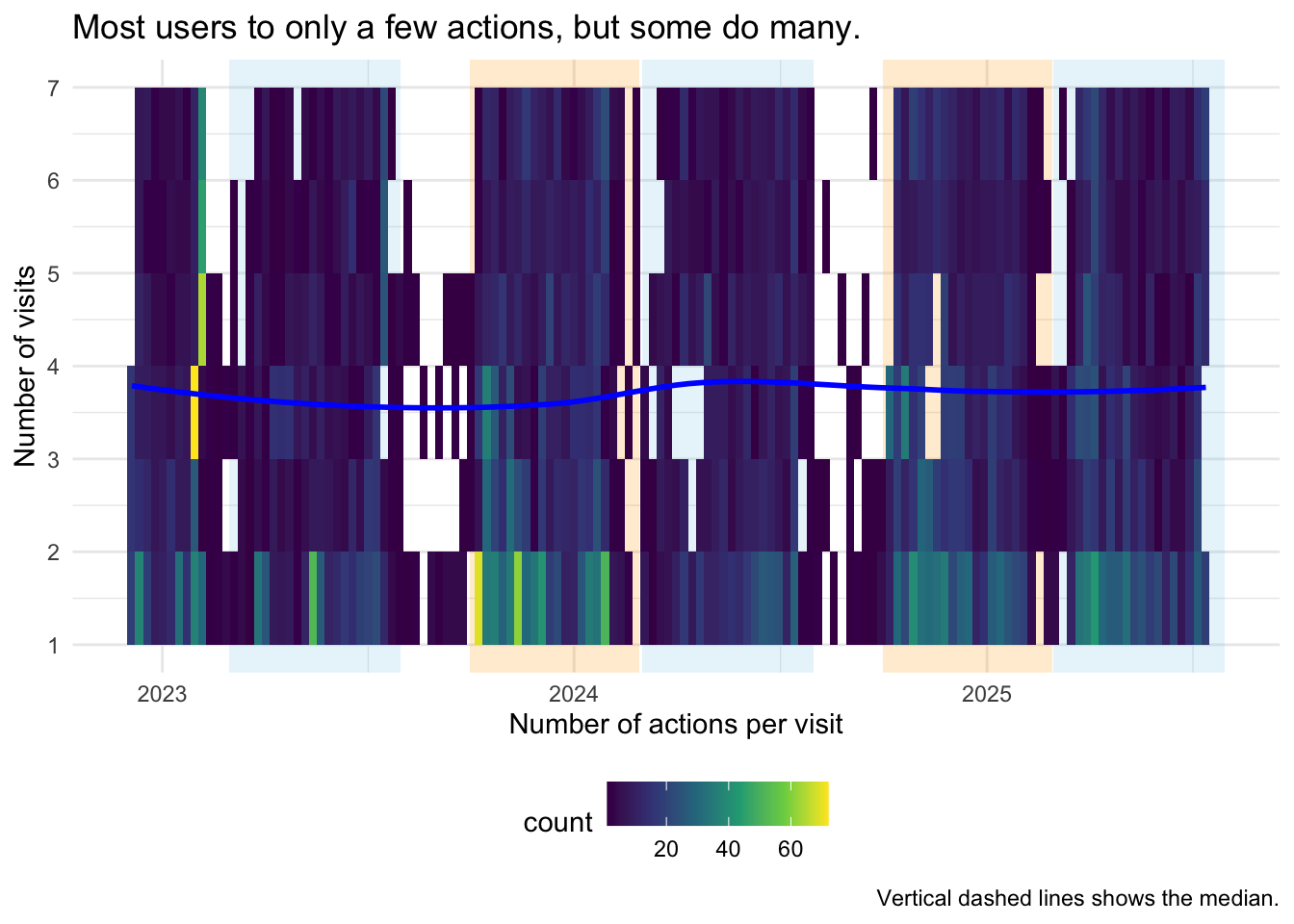
Betrachtet man die Anzahl der Aktionen pro Visit näher, so fällt auf, dass der Maximalwert (499) sehr häufig vorkommt:

Show the code

n_action |>
  count(nr_max) |>
  ggplot(aes(x = nr_max, y = n)) +
  geom_col() +
  geom_vline(
    xintercept = tbl_n_action$Median,
    color = "blue",
    linetype = "dashed"
  ) +
  labs(
    caption = "Vertical dashed lines shows the median.",
    title = "Most users do only a few actions, but some do many.",
    x = "Number of actions per visit",
    y = "Number of visits"
  )

Wichtig

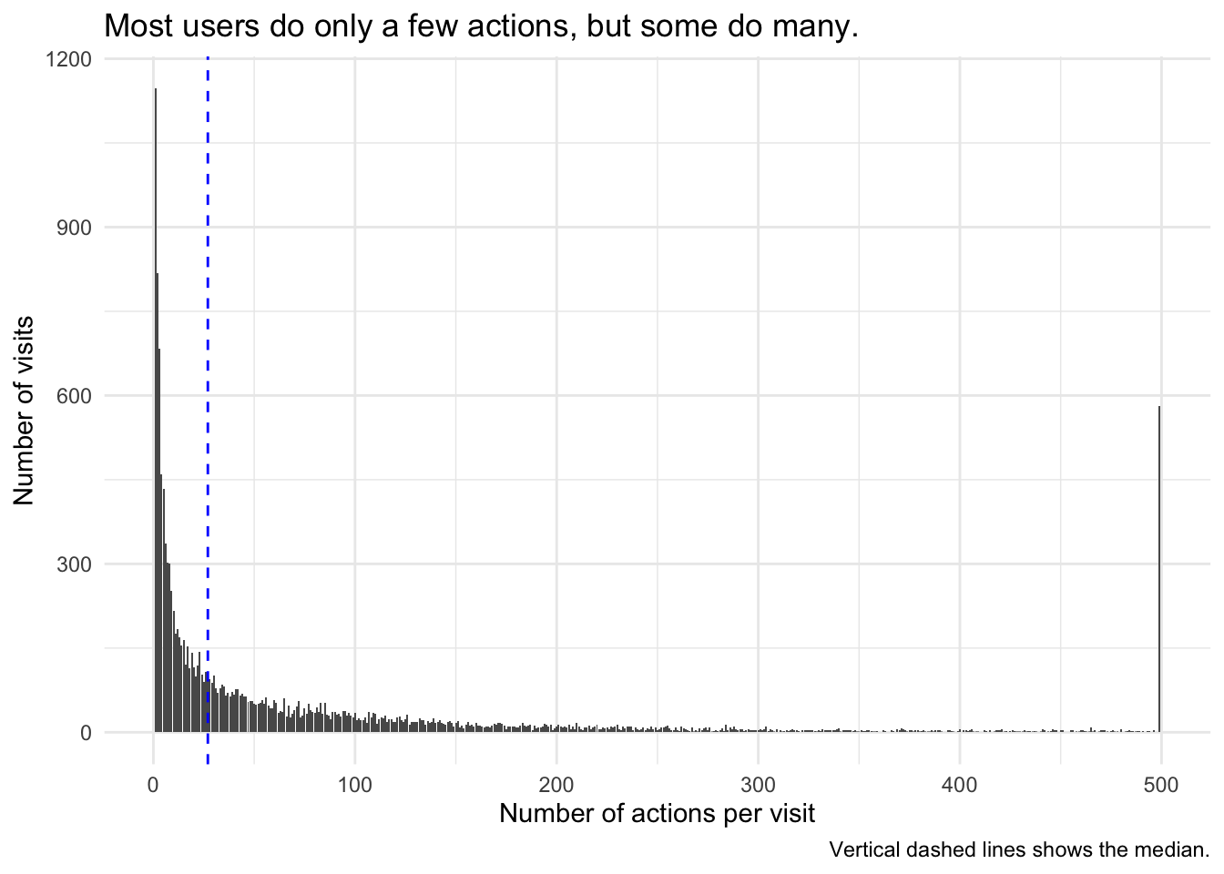
Die meisten Nutzer machen nur wenige Aktionen pro Visit, aber einige machen sehr viele.

Hier noch in einer anderen Darstellung:

Show the code

n_action |>
  count(nr_max) |>
  ggplot(aes(x = nr_max, y = n)) +
  geom_point()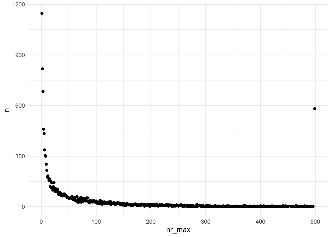

Der Maximalwert ist einfach auffällig häufig:

Show the code

n_action |>
  count(nr_max == 499) |>
  gt()

nr_max == 499	n
FALSE	13626
TRUE	581

Es erscheint plausibel, dass der Maximalwert alle “gekappten” (zensierten, abgeschnittenen) Werte fasst, also viele Werte, die eigentlich größer wären (aber dann zensiert wurden).

3.6.2 fingerprint

Show the code

tbl_n_action_fingerprint <-
  n_action_fingerprint |>
  describe_distribution(nr_max, centrality = c("median", "mean"))

tbl_n_action_fingerprint

Show the code

n_action_fingerprint |>
  count(nr_max) |>
  ggplot(aes(x = nr_max, y = n)) +
  geom_col() +
  geom_vline(
    xintercept = tbl_n_action_fingerprint$Median,
    color = "blue",
    linetype = "dashed"
  ) +
  labs(
    caption = "Vertical dashed lines shows the median.",
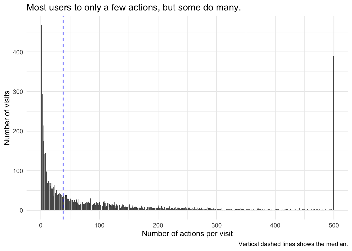
    title = "Most users to only a few actions, but some do many.",
    x = "Number of actions per visit",
    y = "Number of visits"
  )

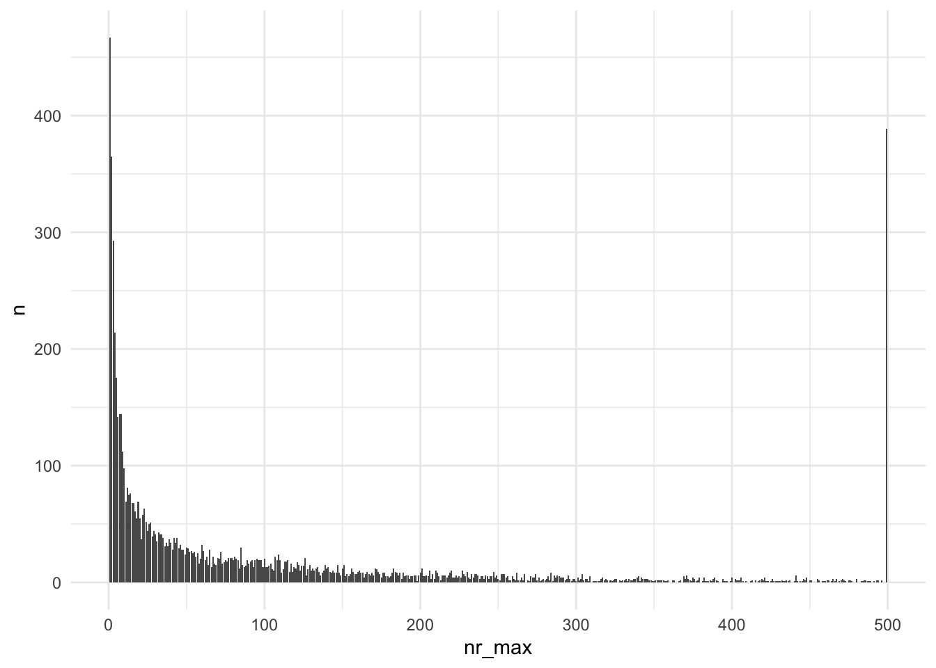
3.6.3 fingerprint unique

Show the code

tbl_n_action_fingerprint_unique <-
  n_action_fingerprint |>
  distinct(fingerprint, .keep_all = TRUE)

tbl_n_action_fingerprint_unique |>
  describe_distribution(nr_max, centrality = c("median", "mean"))

Show the code

tbl_n_action_fingerprint_unique |>
  count(nr_max) |>
  ggplot(aes(x = nr_max, y = n)) +
  geom_col() +
  geom_vline(
    xintercept = tbl_n_action_fingerprint_unique$Median,
    color = "blue",
    linetype = "dashed"
  )

3.7 Nur Visitors, für die weniger als 500 Aktionen protokolliert sind

3.7.1 idvisit

Show the code

n_action_lt_500 |>
  describe_distribution(nr_max) |>
  gt() |>
  fmt_number(columns = where(is.numeric), decimals = 2)

Variable	Mean	SD	IQR	Min	Max	Skewness	Kurtosis	n	n_Missing
nr_max	61.88	88.53	77.00	1.00	496.00	2.27	5.47	13,626.00	0.00

3.7.2 fingerprint

Show the code

n_action_lt_500_fingerprint |>
  describe_distribution(nr_max) |>
  gt() |>
  fmt_number(columns = where(is.numeric), decimals = 2)

Variable	Mean	SD	IQR	Min	Max	Skewness	Kurtosis	n	n_Missing
nr_max	75.78	99.73	100.00	1.00	496.00	1.88	3.31	6,771.00	0.00

3.7.3 fingerprint unique

Show the code

n_action_lt_500_fingerprint_unique <-
  n_action_fingerprint |>
  filter(nr_max != 499) |>
  distinct(fingerprint, .keep_all = TRUE)

n_action_lt_500_fingerprint_unique |>
  describe_distribution(nr_max) |>
  gt() |>
  fmt_number(columns = where(is.numeric), decimals = 2)

Variable	Mean	SD	IQR	Min	Max	Skewness	Kurtosis	n	n_Missing
nr_max	75.78	99.73	100.00	1.00	496.00	1.88	3.31	6,771.00	0.00

3.8 An welchen Tagen und zu welcher Zeit kommen die User zu HaNS?

3.8.1 Setup

3.8.1.1 idvisit

Show the code

# Define a vector with the names of the days of the week
# Note: Adjust the start of the week (Sunday or Monday) as per your requirement
days_of_week <- c(
  "Monday",
  "Tuesday",
  "Wednesday",
  "Thursday",
  "Friday",
  "Saturday",
  "Sunday"
)

# Replace numbers with day names
time_visit_wday$dow2 <- factor(
  days_of_week[time_visit_wday$dow],
  levels = days_of_week
)

3.8.1.2 fingerprint

Show the code

# Define a vector with the names of the days of the week
# Note: Adjust the start of the week (Sunday or Monday) as per your requirement
days_of_week <- c(
  "Monday",
  "Tuesday",
  "Wednesday",
  "Thursday",
  "Friday",
  "Saturday",
  "Sunday"
)

# Replace numbers with day names
time_visit_wday_fingerprint$dow2 <- factor(
  days_of_week[time_visit_wday_fingerprint$dow],
  levels = days_of_week
)

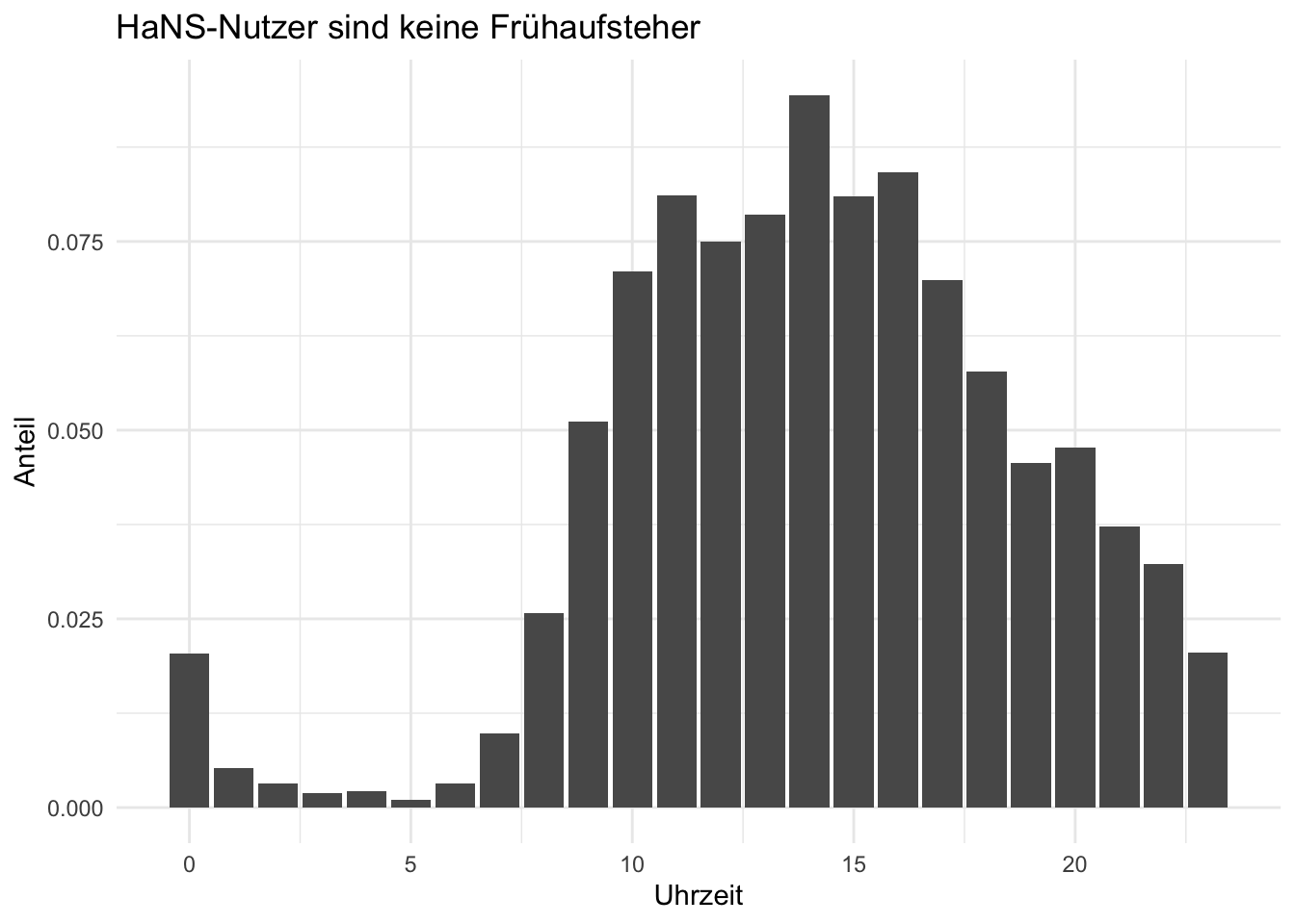
3.8.2 HaNS-Login nach Uhrzeit

3.8.2.1 idvisit

Show the code

time_visit_wday |>
  as_tibble() |>
  count(hour) |>
  mutate(prop = n / sum(n)) |>
  ggplot(aes(x = hour, y = prop)) +
  geom_col() +
  theme_minimal() +
  labs(
    title = "HaNS-Nutzer sind keine Frühaufsteher",
    x = "Uhrzeit",
    y = "Anteil"
  )

Show the code

# coord_polar()

3.8.2.2 fingerprint unique

Show the code

time_visit_wday_summary_fingerprint |>
  as_tibble() |>
  distinct(hour, .keep_all = TRUE) |>
  count(hour) |>
  mutate(prop = n / sum(n)) |>
  ggplot(aes(x = hour, y = prop)) +
  geom_col() +
  theme_minimal() +
  labs(
    title = "HaNS-Nutzer sind keine Frühaufsteher",
    x = "Uhrzeit",
    y = "Anteil"
  )

Show the code

# coord_polar()

Show the code

time_visit_wday |>
  as_tibble() |>
  count(hour) |>
  mutate(prop = n / sum(n)) |>
  ggplot(aes(x = hour, y = prop)) +
  geom_col() +
  theme_minimal() +
  coord_polar()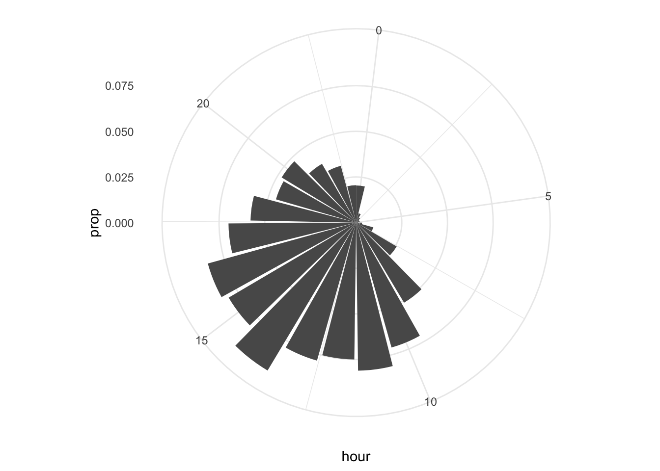

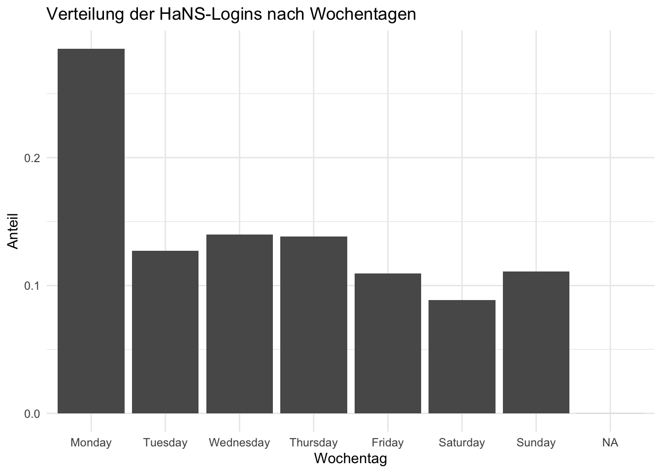
3.8.3 Verteilung der HaNS-Besuche nach Wochentagen

3.8.3.1 idvisit

Show the code

time_visit_wday |>
  as_tibble() |>
  count(dow2) |>
  mutate(prop = n / sum(n)) |>
  ggplot(aes(x = dow2, y = prop)) +
  geom_col() +
  theme_minimal() +
  labs(
    title = "Verteilung der HaNS-Logins nach Wochentagen",
    x = "Wochentag",
    y = "Anteil"
  )

Show the code

# coord_polar()

Show the code

time_visit_wday |>
  as_tibble() |>
  count(dow2) |>
  mutate(prop = n / sum(n)) |>
  ggplot(aes(x = dow2, y = prop)) +
  geom_col() +
  theme_minimal() +
  labs(
    title = "Verteilung der HaNS-Logins nach Wochentagen",
    x = "Wochentag",
    y = "Anteil"
  ) +
  coord_polar()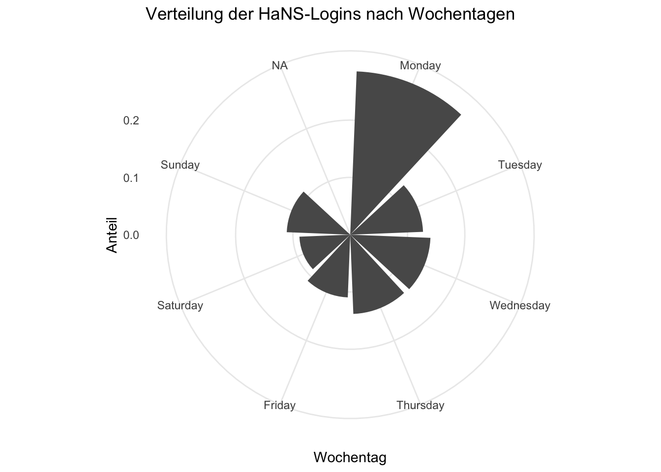

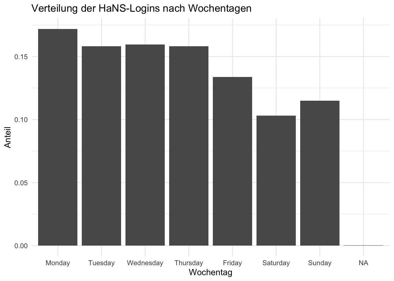
3.8.3.1.1 fingerprint

Show the code

time_visit_wday_fingerprint |>
  as_tibble() |>
  distinct(fingerprint, .keep_all = TRUE) |>
  count(dow2) |>
  mutate(prop = n / sum(n)) |>
  ggplot(aes(x = dow2, y = prop)) +
  geom_col() +
  theme_minimal() +
  labs(
    title = "Verteilung der HaNS-Logins nach Wochentagen",
    x = "Wochentag",
    y = "Anteil"
  )

Show the code

# coord_polar()

Show the code

time_visit_wday_fingerprint |>
  as_tibble() |>
  distinct(fingerprint, .keep_all = TRUE) |>
  count(dow2) |>
  mutate(prop = n / sum(n)) |>
  ggplot(aes(x = dow2, y = prop)) +
  geom_col() +
  theme_minimal() +
  labs(
    title = "Verteilung der HaNS-Logins nach Wochentagen",
    x = "Wochentag",
    y = "Anteil"
  ) +
  coord_polar()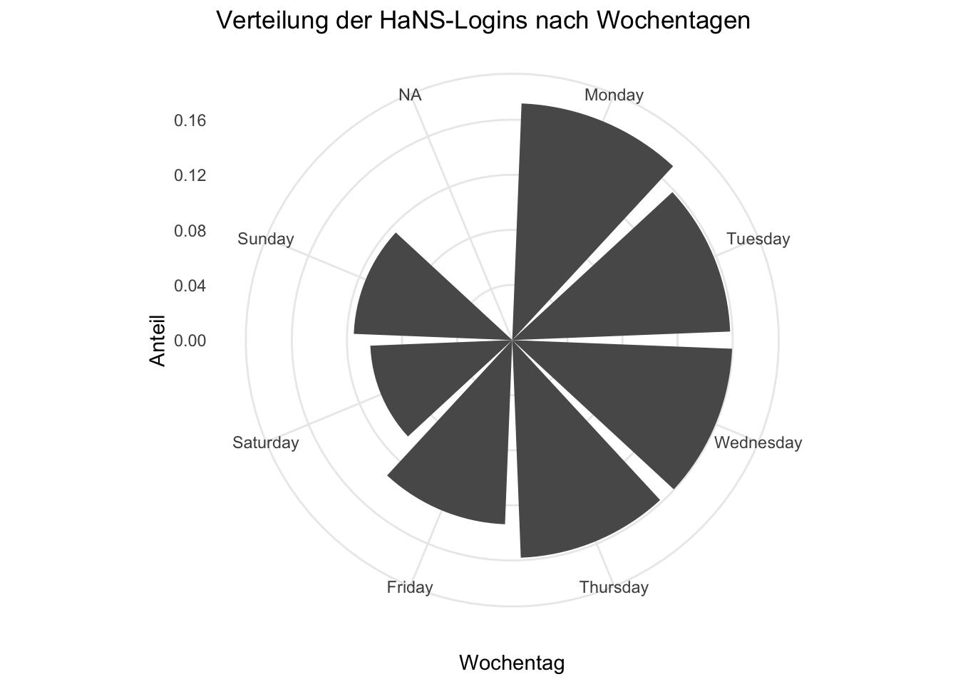

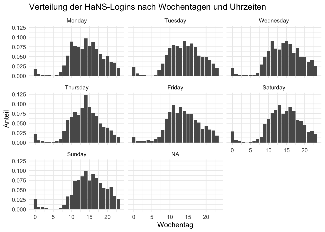
3.8.3.2 HaNS-Login nach Wochentagen Uhrzeit

3.8.3.2.1 idvisit

Show the code

time_visit_wday |>
  as_tibble() |>
  count(dow2, hour) |>
  group_by(dow2) |>
  mutate(prop = n / sum(n)) |>
  ggplot(aes(x = hour, y = prop)) +
  geom_col() +
  facet_wrap(~dow2) +
  theme_minimal() +
  labs(
    title = "Verteilung der HaNS-Logins nach Wochentagen und Uhrzeiten",
    x = "Wochentag",
    y = "Anteil"
  )

Show the code

# coord_polar()

Show the code

time_visit_wday |>
  as_tibble() |>
  count(dow2, hour) |>
  group_by(dow2) |>
  mutate(prop = n / sum(n)) |>
  ggplot(aes(x = hour, y = prop)) +
  geom_col() +
  facet_wrap(~dow2) +
  theme_minimal() +
  labs(
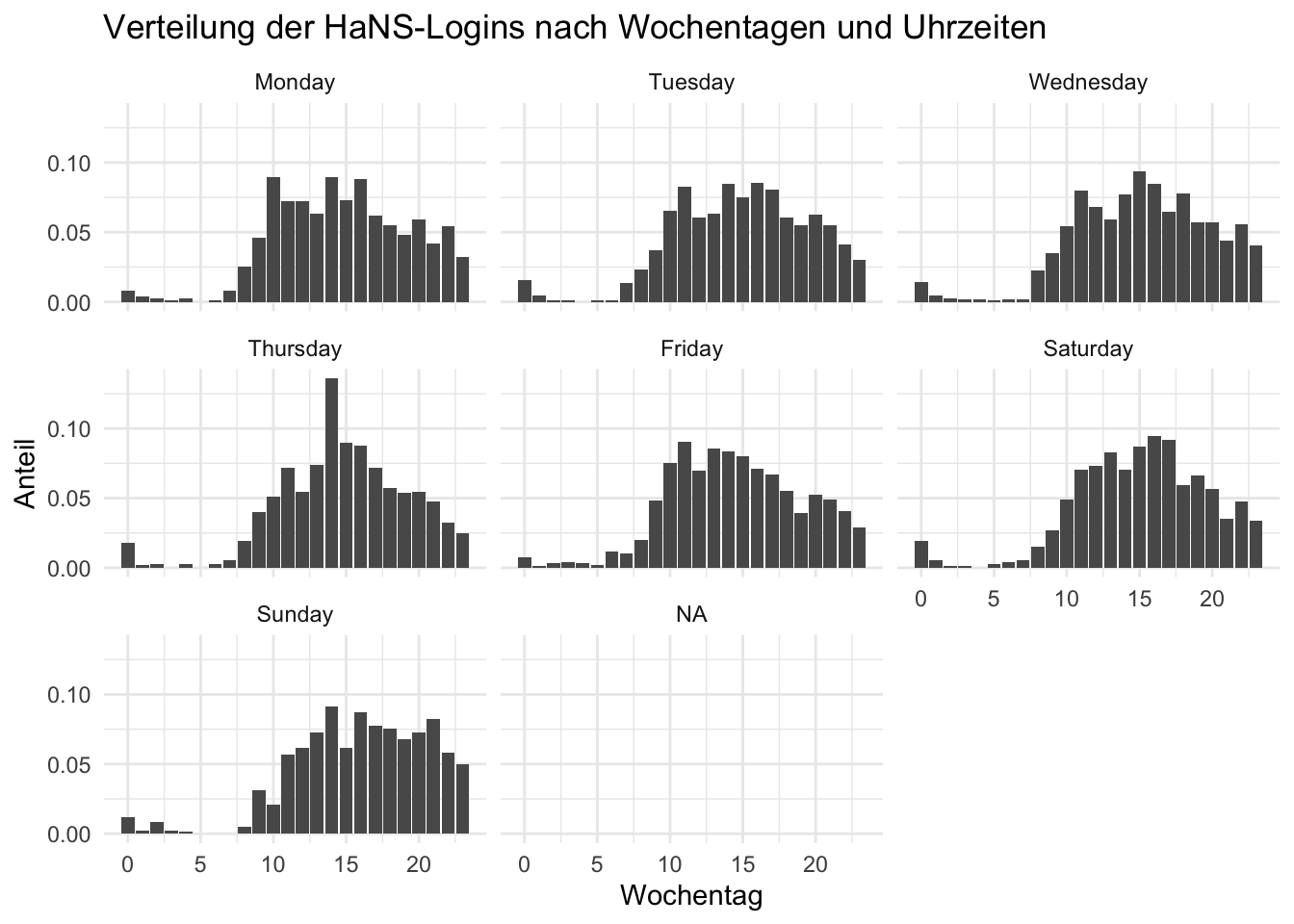
    title = "Verteilung der HaNS-Logins nach Wochentagen und Uhrzeiten",
    x = "Wochentag",
    y = "Anteil"
  ) +
  coord_polar()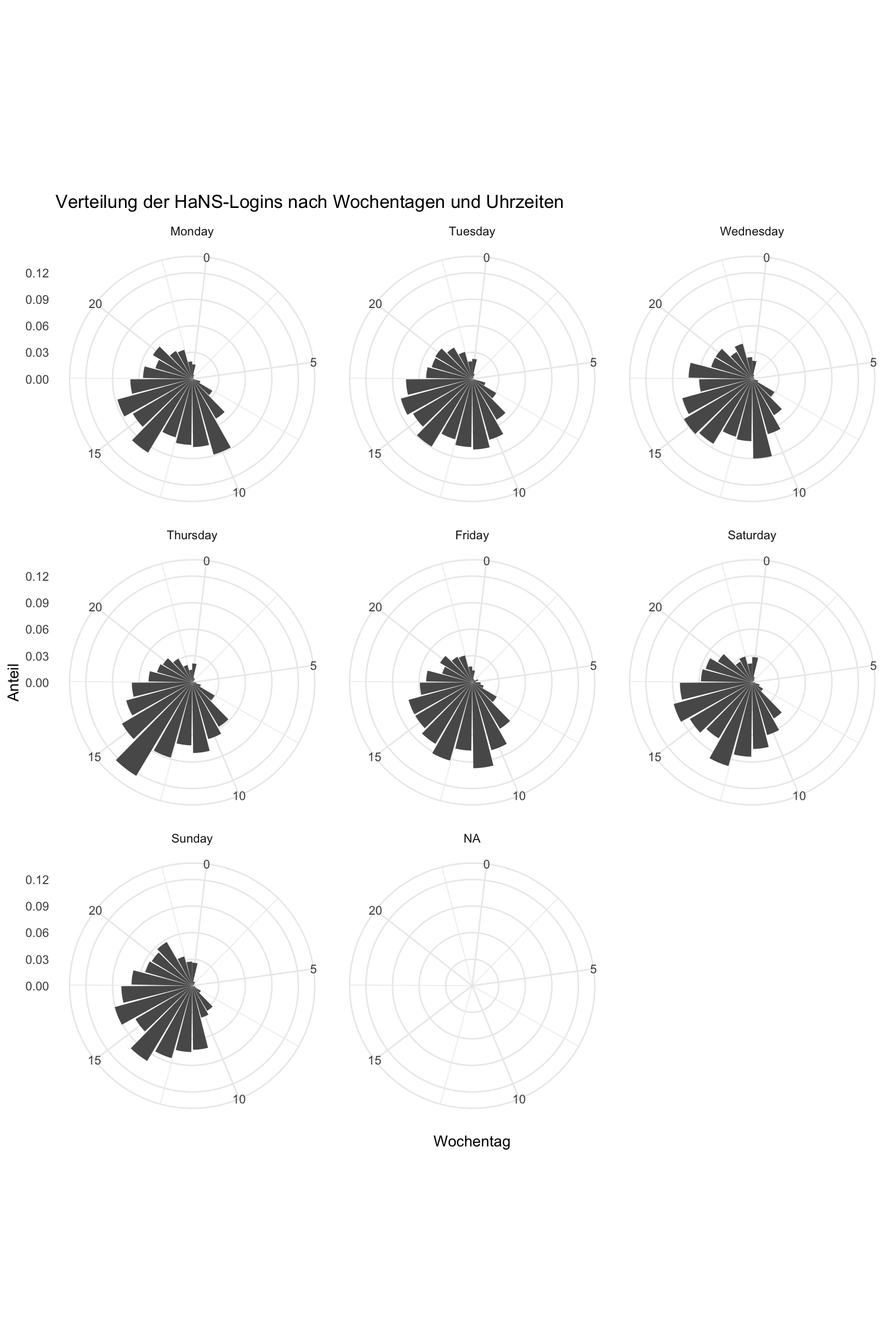

3.8.3.2.2 fingerprint

Show the code

time_visit_wday_fingerprint |>
  as_tibble() |>
  distinct(fingerprint, .keep_all = TRUE) |>
  count(dow2, hour) |>
  group_by(dow2) |>
  mutate(prop = n / sum(n)) |>
  ggplot(aes(x = hour, y = prop)) +
  geom_col() +
  facet_wrap(~dow2) +
  theme_minimal() +
  labs(
    title = "Verteilung der HaNS-Logins nach Wochentagen und Uhrzeiten",
    x = "Wochentag",
    y = "Anteil"
  )

Show the code

# coord_polar()

Show the code

time_visit_wday_fingerprint |>
  as_tibble() |>
  distinct(fingerprint, .keep_all = TRUE) |>
  count(dow2, hour) |>
  group_by(dow2) |>
  mutate(prop = n / sum(n)) |>
  ggplot(aes(x = hour, y = prop)) +
  geom_col() +
  facet_wrap(~dow2) +
  theme_minimal() +
  labs(
    title = "Verteilung der HaNS-Logins nach Wochentagen und Uhrzeiten",
    x = "Wochentag",
    y = "Anteil"
  ) +
  coord_polar()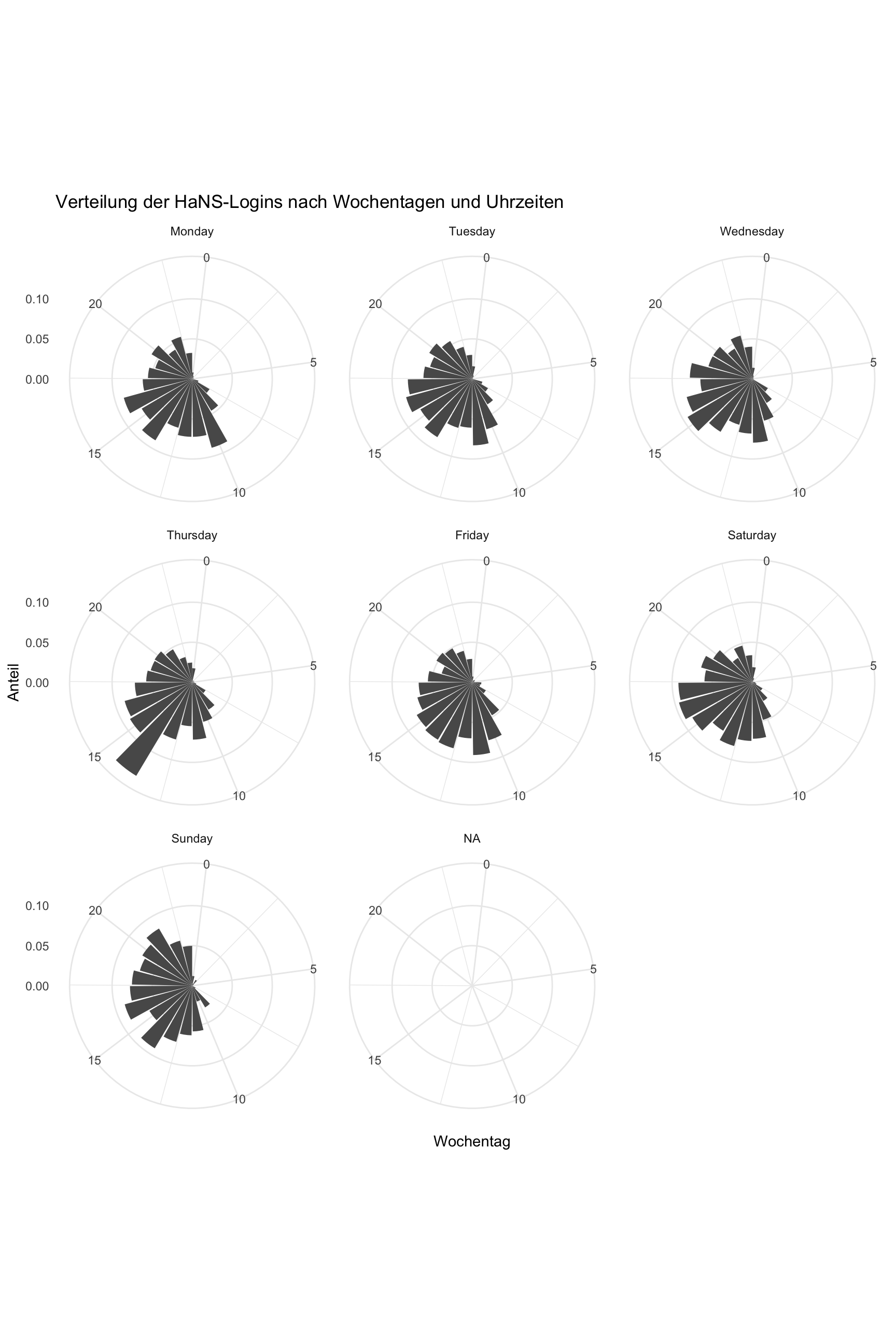

3.8.4 Anzahl der Visits nach Datum (Tagen) und Uhrzeit (bin2d)

3.8.4.1 idvisit

Show the code

time2 <-
  time_visit_wday |>
  ungroup() |>
  mutate(date = as.Date(date_time)) |>
  mutate(month_start = floor_date(date_time, "month"))

time2 |>
  ggplot(aes(x = date, y = hour)) +
  geom_bin2d(binwidth = c(1, 1)) + # (1 day, 1 hour)
  scale_x_date(date_breaks = "1 month") +
  theme(legend.position = "bottom") +
  scale_fill_viridis_c() +
  labs(caption = "Each x-bin maps to one week") +
  scale_x_date(breaks = breaks_pretty()) +
  labs(
    caption = "Vertical dashed lines shows the median.",
    title = "Most users to only a few actions, but some do many.",
    x = "Number of actions per visit",
    y = "Number of visits"
  ) +

  # --- Highlight March–July (approx 1 Mar to 31 Jul) ---
  annotate(
    "rect",
    xmin = as.Date("2023-03-01"),
    xmax = as.Date("2023-07-31"),
    ymin = -Inf,
    ymax = Inf,
    alpha = 0.2,
    fill = "skyblue"
  ) +

  annotate(
    "rect",
    xmin = as.Date("2024-03-01"),
    xmax = as.Date("2024-07-31"),
    ymin = -Inf,
    ymax = Inf,
    alpha = 0.2,
    fill = "skyblue"
  ) +
  annotate(
    "rect",
    xmin = as.Date("2025-03-01"),
    xmax = as.Date("2025-07-31"),
    ymin = -Inf,
    ymax = Inf,
    alpha = 0.2,
    fill = "skyblue"
  ) +

  # --- Highlight October–February (semester break or 2nd term) ---
  annotate(
    "rect",
    xmin = as.Date("2023-10-01"),
    xmax = as.Date("2024-02-28"),
    ymin = -Inf,
    ymax = Inf,
    alpha = 0.2,
    fill = "orange"
  ) +
  # annotate("rect",
  #          xmin = as.Date("2024-10-01"), xmax = as.Date("2024-02-28"),
  #          ymin = -Inf, ymax = Inf, alpha = 0.2, fill = "orange") +
  annotate(
    "rect",
    xmin = as.Date("2024-10-01"),
    xmax = as.Date("2025-02-28"),
    ymin = -Inf,
    ymax = Inf,
    alpha = 0.2,
    fill = "orange"
  )  +
  geom_smooth(method = "loess", se = FALSE, color = "blue")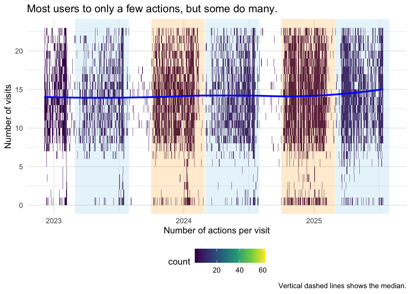

3.8.4.2 fingerprint unique

Show the code

time2_fingerprint <-
  time_visit_wday_fingerprint |>
  ungroup() |>
  distinct(fingerprint, .keep_all = TRUE) |>
  mutate(date = as.Date(date_time)) |>
  mutate(month_start = floor_date(date_time, "month"))

time2_fingerprint |>
  ggplot(aes(x = date, y = hour)) +
  scale_x_date(date_breaks = "1 month") +
  theme(legend.position = "bottom") +
  scale_fill_viridis_c() +
  labs(caption = "Each x-bin maps to one week") +
  scale_x_date(breaks = breaks_pretty()) +
  labs(title = "Visits have increased linearly over time.", x = "month/year") +
  annotate(
    "rect",
    xmin = as.Date("2023-03-01"),
    xmax = as.Date("2023-07-31"),
    ymin = -Inf,
    ymax = Inf,
    alpha = 0.2,
    fill = "skyblue"
  ) +

  annotate(
    "rect",
    xmin = as.Date("2024-03-01"),
    xmax = as.Date("2024-07-31"),
    ymin = -Inf,
    ymax = Inf,
    alpha = 0.2,
    fill = "skyblue"
  ) +
  annotate(
    "rect",
    xmin = as.Date("2025-03-01"),
    xmax = as.Date("2025-07-31"),
    ymin = -Inf,
    ymax = Inf,
    alpha = 0.2,
    fill = "skyblue"
  ) +

  # --- Highlight October–February (semester break or 2nd term) ---
  annotate(
    "rect",
    xmin = as.Date("2023-10-01"),
    xmax = as.Date("2024-02-28"),
    ymin = -Inf,
    ymax = Inf,
    alpha = 0.2,
    fill = "orange"
  ) +
  # annotate("rect",
  #          xmin = as.Date("2024-10-01"), xmax = as.Date("2024-02-28"),
  #          ymin = -Inf, ymax = Inf, alpha = 0.2, fill = "orange") +
  annotate(
    "rect",
    xmin = as.Date("2024-10-01"),
    xmax = as.Date("2025-02-28"),
    ymin = -Inf,
    ymax = Inf,
    alpha = 0.2,
    fill = "orange"
  ) +
  geom_bin2d(binwidth = c(1, 1))  + # (1 day, 1 hour) +
  geom_smooth(method = "loess", se = FALSE, color = "blue")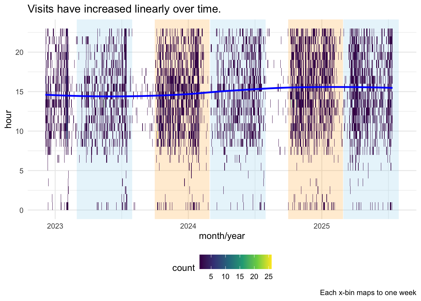

### Anzahl der Visits nach Datum (Wochen) und Uhrzeit (bin2d)

#### idvisit

Show the code

  time2 |>
    ggplot(aes(x = date, y = hour)) +
  scale_x_date(date_breaks = "1 week", date_labels = "%W") +
  theme(legend.position = "bottom") +
  scale_fill_viridis_c() +
  labs(
    x = "Week number in 2023/2024",
    caption = "Each x-bin maps to one week"
  ) +
  scale_x_date(breaks = breaks_pretty())+
  labs(
    caption = "Vertical dashed lines shows the median.",
    title = "Most users to only a few actions, but some do many.",
    x = "Number of actions per visit",
    y = "Number of visits"
  ) +

  # --- Highlight March–July (approx 1 Mar to 31 Jul) ---
  annotate(
    "rect",
    xmin = as.Date("2023-03-01"),
    xmax = as.Date("2023-07-31"),
    ymin = -Inf,
    ymax = Inf,
    alpha = 0.2,
    fill = "skyblue"
  ) +

  annotate(
    "rect",
    xmin = as.Date("2024-03-01"),
    xmax = as.Date("2024-07-31"),
    ymin = -Inf,
    ymax = Inf,
    alpha = 0.2,
    fill = "skyblue"
  ) +
  annotate(
    "rect",
    xmin = as.Date("2025-03-01"),
    xmax = as.Date("2025-07-31"),
    ymin = -Inf,
    ymax = Inf,
    alpha = 0.2,
    fill = "skyblue"
  ) +

  # --- Highlight October–February (semester break or 2nd term) ---
  annotate(
    "rect",
    xmin = as.Date("2023-10-01"),
    xmax = as.Date("2024-02-28"),
    ymin = -Inf,
    ymax = Inf,
    alpha = 0.2,
    fill = "orange"
  ) +
  # annotate("rect",
  #          xmin = as.Date("2024-10-01"), xmax = as.Date("2024-02-28"),
  #          ymin = -Inf, ymax = Inf, alpha = 0.2, fill = "orange") +
  annotate(
    "rect",
    xmin = as.Date("2024-10-01"),
    xmax = as.Date("2025-02-28"),
    ymin = -Inf,
    ymax = Inf,
    alpha = 0.2,
    fill = "orange"
  )+
  geom_bin2d(binwidth = c(7, 1)) + # 1 week, 1 hour
  geom_smooth(method = "loess", se = FALSE, color = "blue")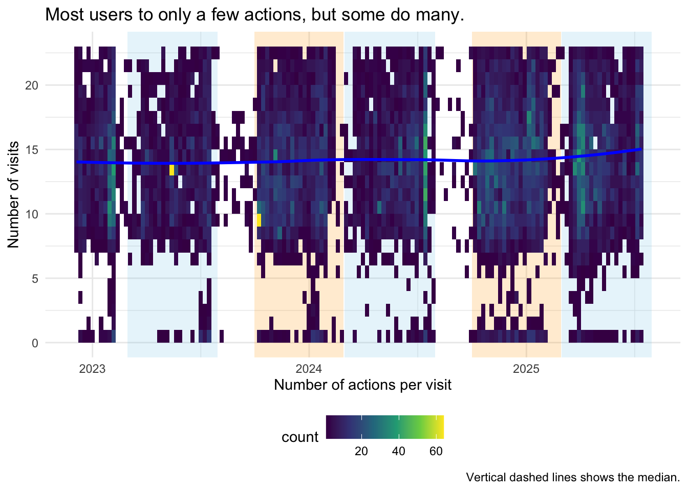

3.8.4.3 fingerprint

Show the code

time2_fingerprint |>
  distinct(fingerprint, .keep_all = TRUE) |>
  ggplot(aes(x = date, y = hour)) +
  scale_x_date(date_breaks = "1 week", date_labels = "%W") +
  theme(legend.position = "bottom") +
  scale_fill_viridis_c() +
  labs(
    x = "Week number in 2023/2024",
    caption = "Each x-bin maps to one week"
  ) +
  scale_x_date(breaks = breaks_pretty())+
  labs(
    caption = "Vertical dashed lines shows the median.",
    title = "Most users to only a few actions, but some do many.",
    x = "Number of actions per visit",
    y = "Number of visits"
  ) +

  # --- Highlight March–July (approx 1 Mar to 31 Jul) ---
  annotate(
    "rect",
    xmin = as.Date("2023-03-01"),
    xmax = as.Date("2023-07-31"),
    ymin = -Inf,
    ymax = Inf,
    alpha = 0.2,
    fill = "skyblue"
  ) +

  annotate(
    "rect",
    xmin = as.Date("2024-03-01"),
    xmax = as.Date("2024-07-31"),
    ymin = -Inf,
    ymax = Inf,
    alpha = 0.2,
    fill = "skyblue"
  ) +
  annotate(
    "rect",
    xmin = as.Date("2025-03-01"),
    xmax = as.Date("2025-07-31"),
    ymin = -Inf,
    ymax = Inf,
    alpha = 0.2,
    fill = "skyblue"
  ) +

  # --- Highlight October–February (semester break or 2nd term) ---
  annotate(
    "rect",
    xmin = as.Date("2023-10-01"),
    xmax = as.Date("2024-02-28"),
    ymin = -Inf,
    ymax = Inf,
    alpha = 0.2,
    fill = "orange"
  ) +
  # annotate("rect",
  #          xmin = as.Date("2024-10-01"), xmax = as.Date("2024-02-28"),
  #          ymin = -Inf, ymax = Inf, alpha = 0.2, fill = "orange") +
  annotate(
    "rect",
    xmin = as.Date("2024-10-01"),
    xmax = as.Date("2025-02-28"),
    ymin = -Inf,
    ymax = Inf,
    alpha = 0.2,
    fill = "orange"
  ) + 
  geom_smooth(method = "loess", se = FALSE, color = "blue")+ 
  geom_bin2d(binwidth = c(7, 1))  # 1 week, 1 hour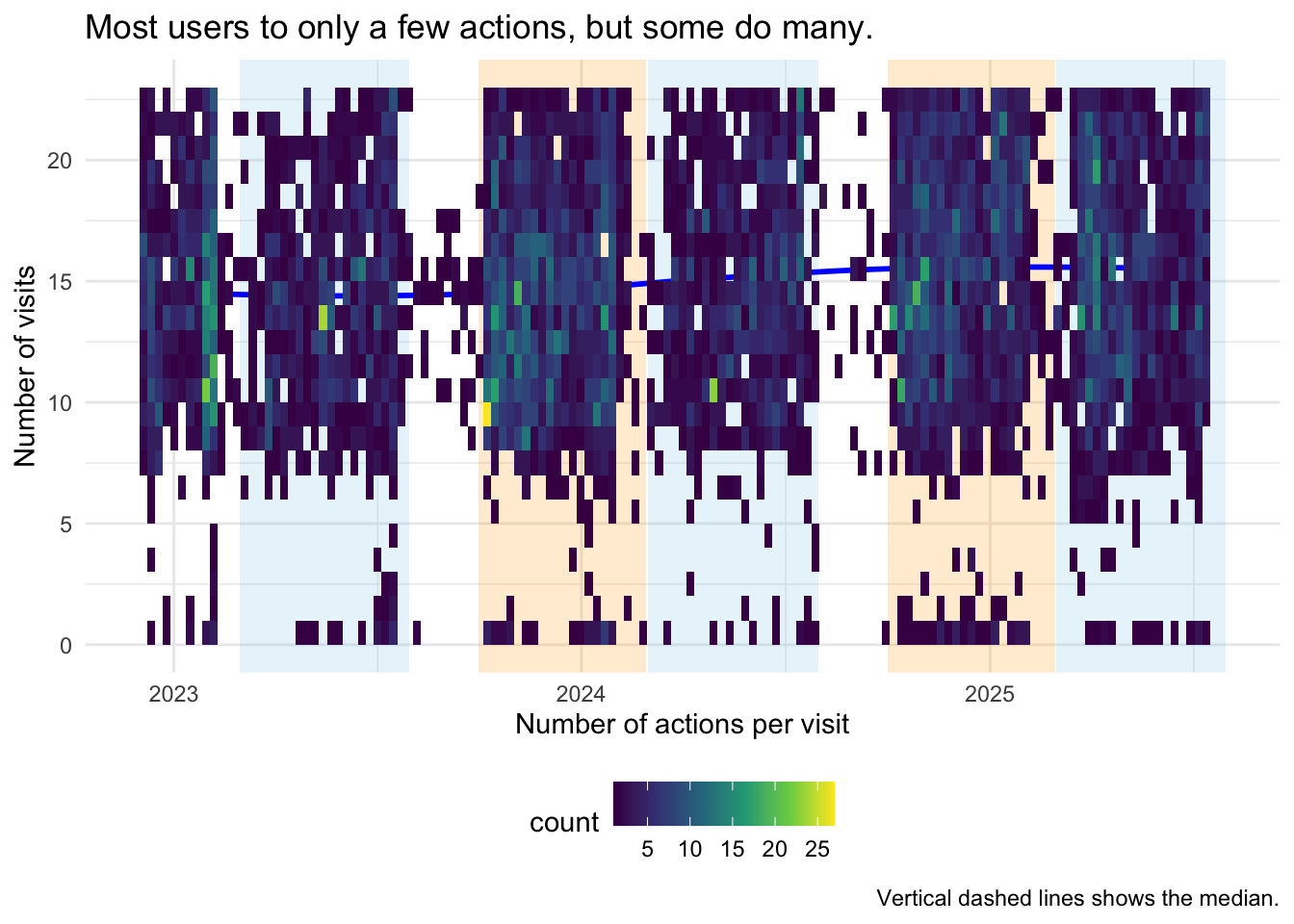

3.8.5 Anzahl der Visits nach Datum (Wochen) und Wochentag (bin2d)

3.8.5.1 idvisit

Show the code

time2 |>
  ggplot(aes(x = date, y = dow)) +
  geom_bin2d(binwidth = c(7, 1)) + # 1 week, 1 hour
  scale_x_date(date_breaks = "1 week", date_labels = "%W") +
  theme(legend.position = "bottom") +
  scale_fill_viridis_c() +
  labs(
    x = "Week number in 2023/2024",
    caption = "Each x-bin maps to one week",
    y = "Day of Week"
  ) +
  scale_y_continuous(breaks = 1:7) +
  scale_x_date(breaks = breaks_pretty())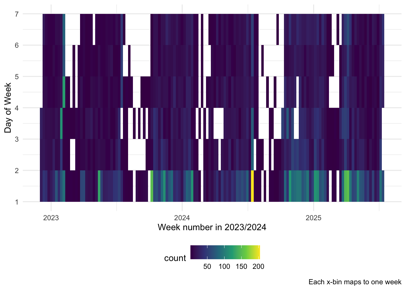

3.8.5.2 fingerprint

Show the code

time2_fingerprint |>
  distinct(fingerprint, .keep_all = TRUE) |>
  ggplot(aes(x = date, y = dow)) +
  scale_x_date(date_breaks = "1 week", date_labels = "%W") +
  theme(legend.position = "bottom") +
  scale_fill_viridis_c() +
  labs(
    x = "Week number in 2023/2024",
    caption = "Each x-bin maps to one week",
    y = "Day of Week"
  ) +
  scale_y_continuous(breaks = 1:7) +
  scale_x_date(breaks = breaks_pretty()) +
  labs(
    caption = "Vertical dashed lines shows the median.",
    title = "Most users to only a few actions, but some do many.",
    x = "Number of actions per visit",
    y = "Number of visits"
  ) +

  # --- Highlight March–July (approx 1 Mar to 31 Jul) ---
  annotate(
    "rect",
    xmin = as.Date("2023-03-01"),
    xmax = as.Date("2023-07-31"),
    ymin = -Inf,
    ymax = Inf,
    alpha = 0.2,
    fill = "skyblue"
  ) +

  annotate(
    "rect",
    xmin = as.Date("2024-03-01"),
    xmax = as.Date("2024-07-31"),
    ymin = -Inf,
    ymax = Inf,
    alpha = 0.2,
    fill = "skyblue"
  ) +
  annotate(
    "rect",
    xmin = as.Date("2025-03-01"),
    xmax = as.Date("2025-07-31"),
    ymin = -Inf,
    ymax = Inf,
    alpha = 0.2,
    fill = "skyblue"
  ) +

  # --- Highlight October–February (semester break or 2nd term) ---
  annotate(
    "rect",
    xmin = as.Date("2023-10-01"),
    xmax = as.Date("2024-02-28"),
    ymin = -Inf,
    ymax = Inf,
    alpha = 0.2,
    fill = "orange"
  ) +
  # annotate("rect",
  #          xmin = as.Date("2024-10-01"), xmax = as.Date("2024-02-28"),
  #          ymin = -Inf, ymax = Inf, alpha = 0.2, fill = "orange") +
  annotate(
    "rect",
    xmin = as.Date("2024-10-01"),
    xmax = as.Date("2025-02-28"),
    ymin = -Inf,
    ymax = Inf,
    alpha = 0.2,
    fill = "orange"
  )  +

  geom_bin2d(binwidth = c(7, 1)) + # 1 week, 1 hour
  geom_smooth(method = "loess", se = FALSE, color = "blue")