n_action_avg=mean(n_action$nr_max)|>round(0)n_action_median=median(n_action$nr_max)|>round(0)n_action_sd=sd(n_action$nr_max)|>round(0)n_action_iqr=IQR(n_action$nr_max)|>round(0)n_action|>ggplot()+geom_histogram(aes(x =nr_max))+labs( x ="Anzahl von Aktionen pro Visit", y ="n", caption ="Der vertikale Strich zeigt den Mittelwert; der horizontale MW±SD")+theme_minimal()+geom_vline(xintercept =n_action_avg, color =palette_okabe_ito()[1])+geom_segment( x =n_action_avg-n_action_sd, y =0, xend =n_action_avg+n_action_sd, yend =0, color =palette_okabe_ito()[2], size =2)+annotate("label", x =n_action_avg, y =1500, label =paste0("MW = ", n_action_avg))+annotate("label", x =n_action_avg+n_action_sd, y =0, label =paste0("SD = ", n_action_sd))
Show the code
#geom_label(aes(x = n_action_avg), y = 1, label = "Mean")n_action|>ggplot()+geom_histogram(aes(x =nr_max))+labs( x ="Anzahl von Aktionen pro Visit", y ="n", caption ="Der vertikale Strich zeigt den Median; der horizontale Median±IQR")+theme_minimal()+geom_vline(xintercept =n_action_median, color =palette_okabe_ito()[1])+geom_segment( x =n_action_median-n_action_iqr, y =0, xend =n_action_median+n_action_iqr, yend =0, color =palette_okabe_ito()[2], size =2)+annotate("label", x =n_action_median, y =1500, label =paste0("Md = ", n_action_median))+annotate("label", x =n_action_median+n_action_iqr, y =0, label =paste0("IQR = ", n_action_iqr))
Show the code
#geom_label(aes(x = n_action_avg), y = 1, label = "Mean")
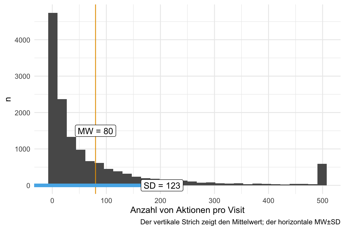
Mittelwert der Aktionen pro Visit: 80.
SD der Aktionen pro Visit: 123.
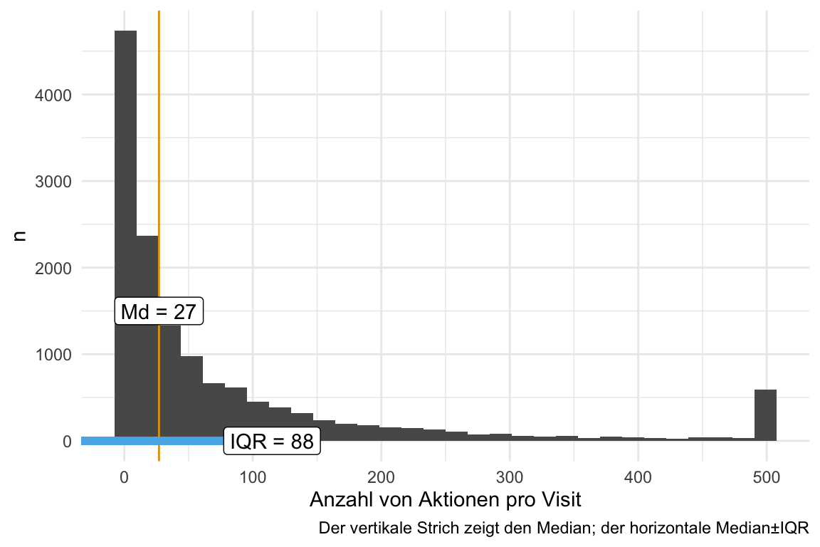
MD: 27.
IQR: : 88.
6.2.2 fingerprint
Show the code
n_action_fingerprint_avg=mean(n_action_fingerprint$nr_max)|>round(0)n_action_fingerprint_median=median(n_action_fingerprint$nr_max)|>round(0)n_action_fingerprint_sd=sd(n_action_fingerprint$nr_max)|>round(0)n_action_fingerprint_iqr=IQR(n_action_fingerprint$nr_max)|>round(0)n_action_fingerprint|>ggplot()+geom_histogram(aes(x =nr_max))+labs( x ="Anzahl von Aktionen pro Visit", y ="n", caption ="Der vertikale Strich zeigt den Mittelwert; der horizontale MW±SD")+theme_minimal()+geom_vline( xintercept =n_action_fingerprint_avg, color =palette_okabe_ito()[1])+geom_segment( x =n_action_fingerprint_avg-n_action_fingerprint_sd, y =0, xend =n_action_fingerprint_avg+n_action_fingerprint_sd, yend =0, color =palette_okabe_ito()[2], size =2)+annotate("label", x =n_action_fingerprint_avg, y =1500, label =paste0("MW = ", n_action_fingerprint_avg))+annotate("label", x =n_action_fingerprint_avg+n_action_fingerprint_sd, y =0, label =paste0("SD = ", n_action_fingerprint_sd))
Show the code
#geom_label(aes(x = n_action_fingerprint_avg), y = 1, label = "Mean")n_action_fingerprint|>ggplot()+geom_histogram(aes(x =nr_max))+labs( x ="Anzahl von Aktionen pro Visit", y ="n", caption ="Der vertikale Strich zeigt den Median; der horizontale Median±IQR")+theme_minimal()+geom_vline( xintercept =n_action_fingerprint_median, color =palette_okabe_ito()[1])+geom_segment( x =n_action_fingerprint_median-n_action_fingerprint_iqr, y =0, xend =n_action_fingerprint_median+n_action_fingerprint_iqr, yend =0, color =palette_okabe_ito()[2], size =2)+annotate("label", x =n_action_fingerprint_median, y =1500, label =paste0("Md = ", n_action_fingerprint_median))+annotate("label", x =n_action_fingerprint_median+n_action_fingerprint_iqr, y =0, label =paste0("IQR = ", n_action_fingerprint_iqr))
Show the code
#geom_label(aes(x = n_action_fingerprint_avg), y = 1, label = "Mean")
6.3 Ohne 499er-Daten
6.3.1 idvisit
Show the code
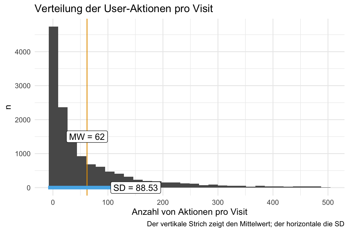
n_action_avg2=mean(n_action_lt_500$nr_max)|>round(0)n_action_sd2=sd(n_action_lt_500$nr_max)|>round(2)n_action_lt_500|>ggplot()+geom_histogram(aes(x =nr_max))+labs( x ="Anzahl von Aktionen pro Visit", y ="n", title ="Verteilung der User-Aktionen pro Visit", caption ="Der vertikale Strich zeigt den Mittelwert; der horizontale die SD")+theme_minimal()+geom_vline(xintercept =n_action_avg2, color =palette_okabe_ito()[1])+geom_segment( x =n_action_avg-n_action_sd2, y =0, xend =n_action_avg2+n_action_sd2, yend =0, color =palette_okabe_ito()[2], size =2)+annotate("label", x =n_action_avg2, y =1500, label =paste0("MW = ", n_action_avg2))+annotate("label", x =n_action_avg2+n_action_sd2, y =0, label =paste0("SD = ", n_action_sd2))
Show the code
#geom_label(aes(x = n_action_avg), y = 1, label = "Mean")
Mittelwert der Aktionen pro Visit: 62.
SD der Aktionen pro Visit: 88.53.
6.3.2 fingerprint unique
Show the code
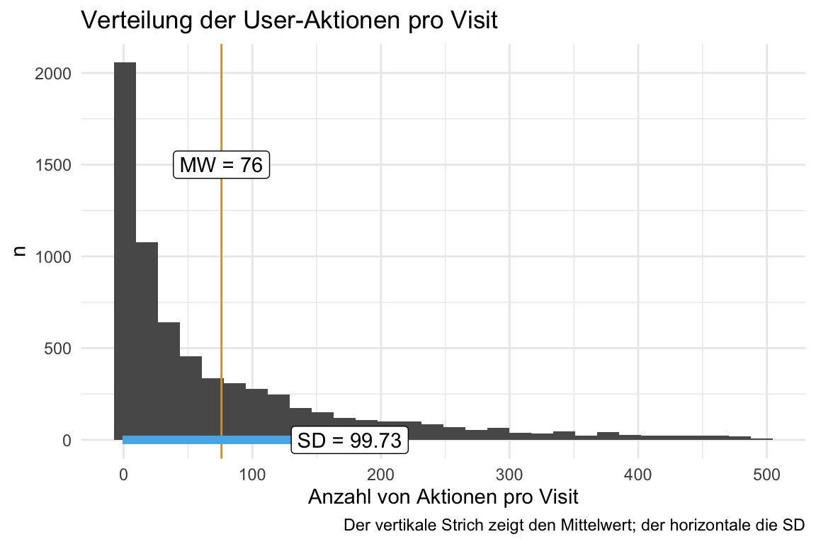
n_action_fingerprint_avg2=mean(n_action_lt_500_fingerprint_unique$nr_max)|>round(0)n_action_fingerprint_sd2=sd(n_action_lt_500_fingerprint_unique$nr_max)|>round(2)n_action_lt_500_fingerprint_unique|>ggplot()+geom_histogram(aes(x =nr_max))+labs( x ="Anzahl von Aktionen pro Visit", y ="n", title ="Verteilung der User-Aktionen pro Visit", caption ="Der vertikale Strich zeigt den Mittelwert; der horizontale die SD")+theme_minimal()+geom_vline( xintercept =n_action_fingerprint_avg2, color =palette_okabe_ito()[1])+geom_segment( x =n_action_fingerprint_avg-n_action_fingerprint_sd2, y =0, xend =n_action_fingerprint_avg2+n_action_fingerprint_sd2, yend =0, color =palette_okabe_ito()[2], size =2)+annotate("label", x =n_action_fingerprint_avg2, y =1500, label =paste0("MW = ", n_action_fingerprint_avg2))+annotate("label", x =n_action_fingerprint_avg2+n_action_fingerprint_sd2, y =0, label =paste0("SD = ", n_action_fingerprint_sd2))
Show the code
#geom_label(aes(x = n_action_avg), y = 1, label = "Mean")
6.4 Anzahl Aktionen im Zeitverlauf
6.4.1 Monat
6.4.1.1 idvisit
Show the code
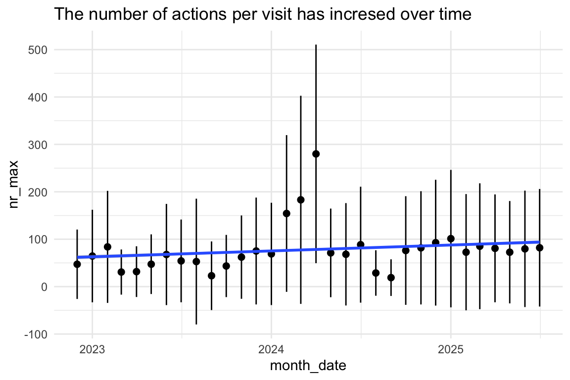
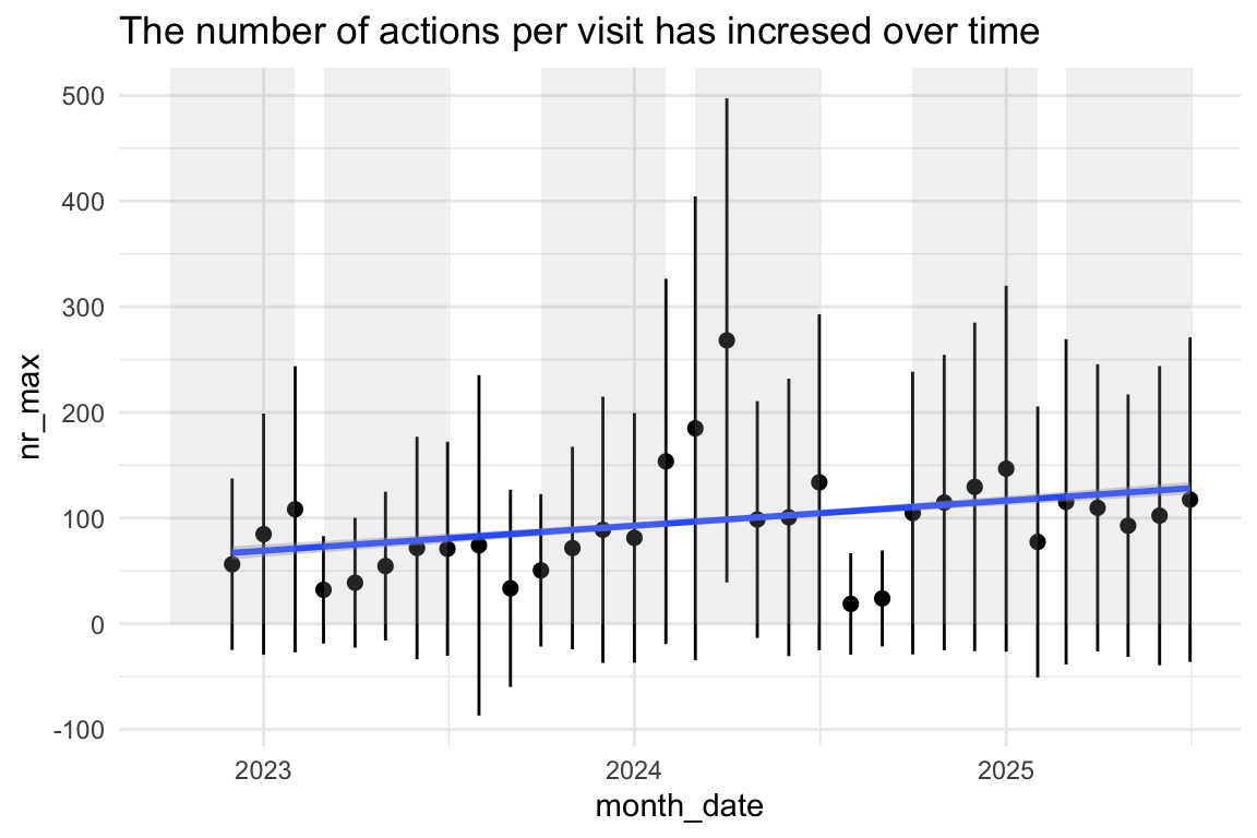
n_action_w_date|>ggplot(aes(x =month_date, y =nr_max))+stat_summary(fun =mean, geom ="point", size =2)+stat_summary( fun.data =mean_sdl, fun.args =list(mult =1), geom ="errorbar", width =0.2)+geom_smooth(method ="lm")+labs(title ="The number of actions per visit has incresed over time")
n_action_w_date_fingerprint_unique<-n_action_w_date_fingerprint|>distinct(fingerprint, .keep_all =TRUE)rect_data<-comp_semester_rects(n_action_w_date_fingerprint_unique, col_date ="month_date")n_action_w_date_fingerprint_unique|>ggplot(aes(x =month_date, y =nr_max))+stat_summary(fun =mean, geom ="point", size =2)+stat_summary( fun.data =mean_sdl, fun.args =list(mult =1), geom ="errorbar", width =0.2)+geom_smooth(method ="lm")+labs(title ="The number of actions per visit has incresed over time")+geom_rect( data =rect_data,aes(xmin =xmin, xmax =xmax, ymin =ymin, ymax =ymax), fill ="grey", alpha =0.2, inherit.aes =FALSE# Essential to use the rect_data columns)
Show the code
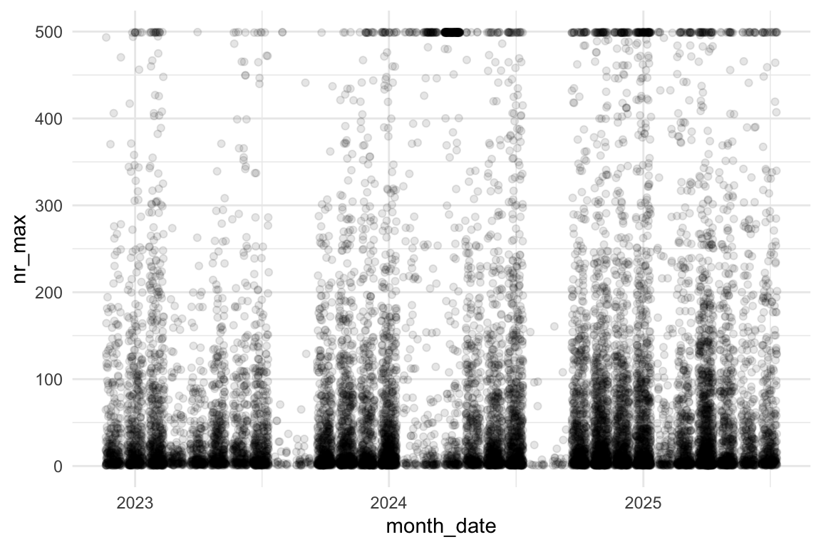
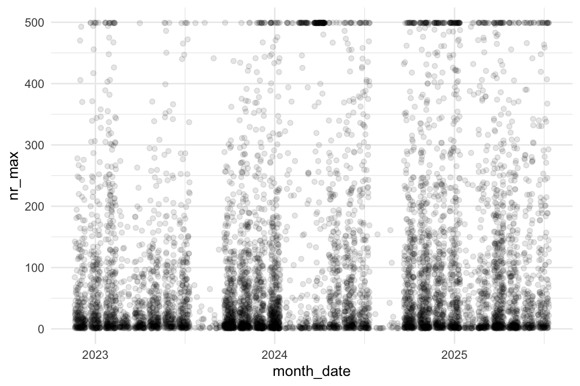
n_action_w_date_fingerprint_unique|>ggplot(aes(x =month_date, y =nr_max))+geom_jitter(alpha =.1)
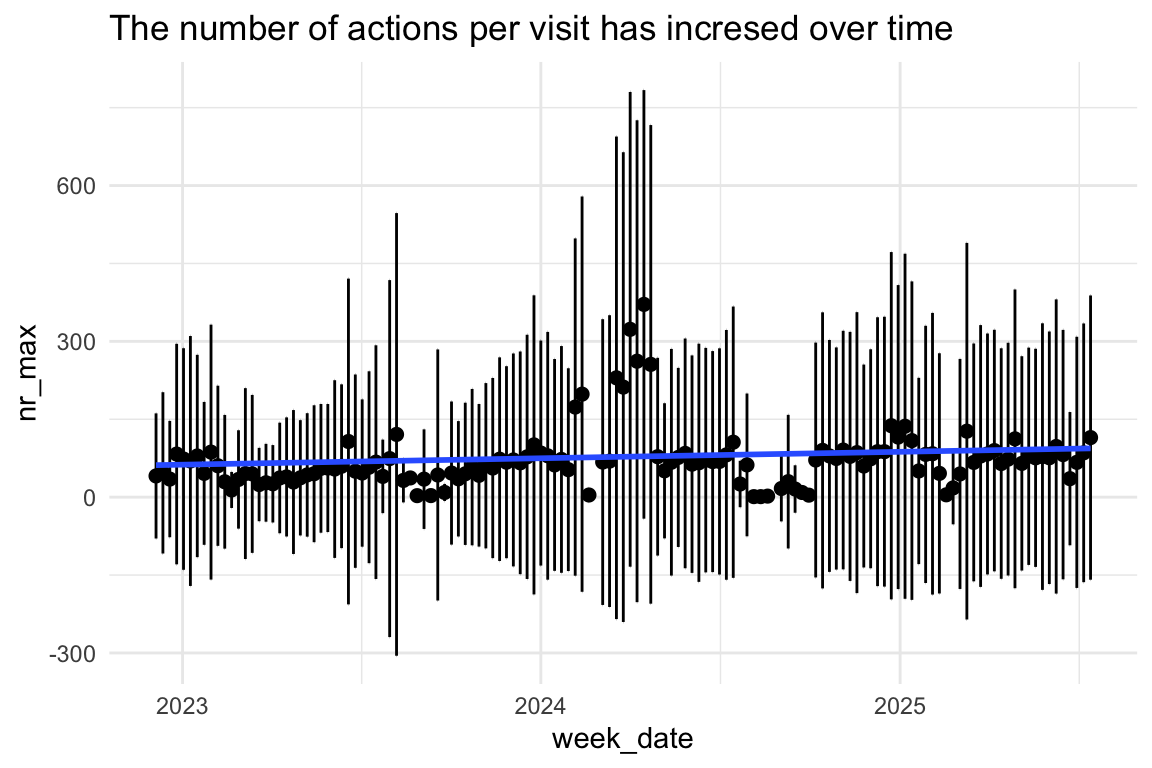
n_action_w_date|>mutate(week_date =as.Date(week_date))|>ggplot(aes(x =week_date, y =nr_max))+stat_summary(fun =mean, geom ="point", size =2)+stat_summary(fun.data =mean_sdl, geom ="errorbar", width =0.2)+geom_smooth(method ="lm")+labs(title ="The number of actions per visit has incresed over time")
6.4.3.2 fingerprint
Show the code
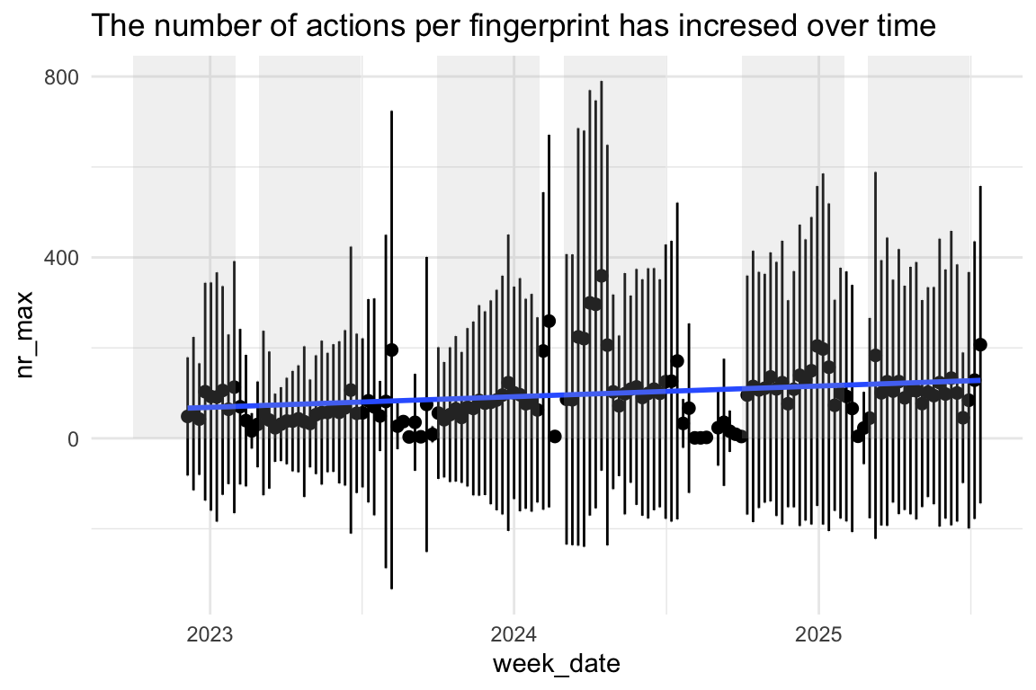
n_action_w_date_fingerprint|>mutate(week_date =as.Date(week_date))|>ggplot(aes(x =week_date, y =nr_max))+stat_summary(fun =mean, geom ="point", size =2)+stat_summary(fun.data =mean_sdl, geom ="errorbar", width =0.2)+geom_smooth(method ="lm")+labs(title ="The number of actions per fingerprint has incresed over time")+geom_rect( data =rect_data,aes(xmin =xmin, xmax =xmax, ymin =ymin, ymax =ymax), fill ="grey", alpha =0.2, inherit.aes =FALSE# Essential to use the rect_data columns)
6.4.3.3 fingerprint unique
Show the code
n_action_w_date_fingerprint_unique<-n_action_w_date_fingerprint|>distinct(fingerprint, .keep_all =TRUE)n_action_w_date_fingerprint_unique|>mutate(week_date =as.Date(week_date))|>ggplot(aes(x =week_date, y =nr_max))+stat_summary(fun =mean, geom ="point", size =2)+stat_summary(fun.data =mean_sdl, geom ="errorbar", width =0.2)+geom_smooth(method ="lm")+labs(title ="The number of actions per fingerprint has incresed over time")+geom_rect( data =rect_data,aes(xmin =xmin, xmax =xmax, ymin =ymin, ymax =ymax), fill ="grey", alpha =0.2, inherit.aes =FALSE# Essential to use the rect_data columns)
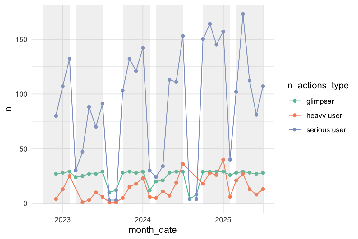
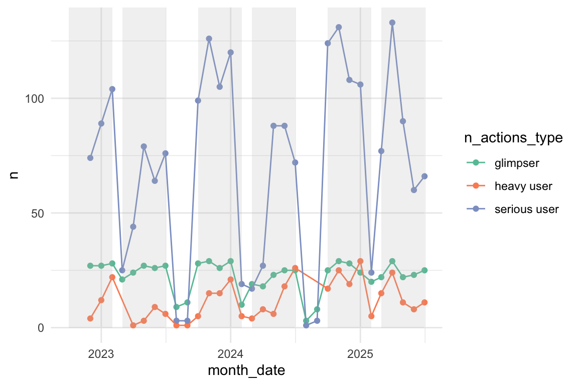
n_action_w_date|>group_by(month_date)|>count(nr_max)|>mutate( n_actions_type =case_when(nr_max<30~"glimpser",nr_max<300~"serious user",TRUE~"heavy user"))|>count(n_actions_type)|>ggplot(aes( x =month_date, y =n, color =n_actions_type, group =n_actions_type))+geom_point()+geom_line()+geom_rect( data =rect_data,aes(xmin =xmin, xmax =xmax, ymin =ymin, ymax =ymax), fill ="grey", alpha =0.2, inherit.aes =FALSE# Essential to use the rect_data columns)
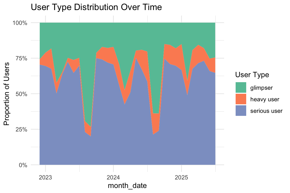
6.7.1.2 Relative Anteile
Show the code
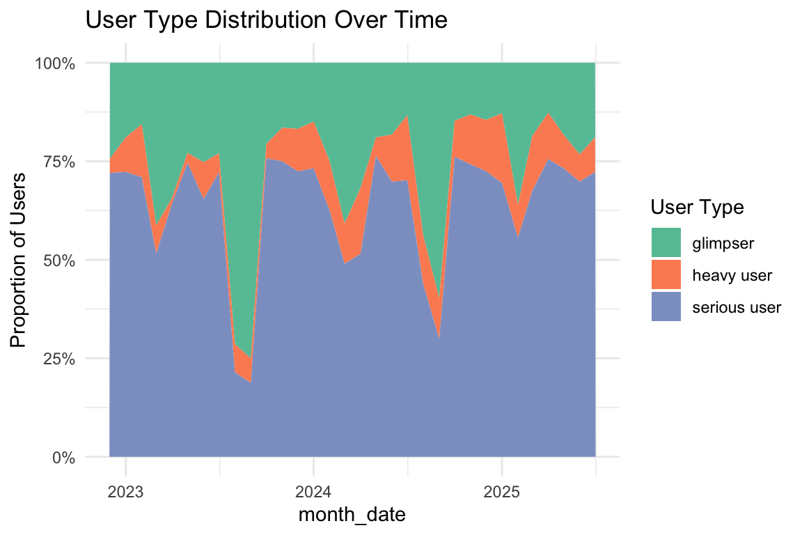
library(data.table)# Ensure data.table is loaded if not alreadylibrary(ggplot2)library(scales)# Needed for label_percent()n_action_w_date|>group_by(month_date)|>count(nr_max)|>mutate( n_actions_type =case_when(nr_max<30~"glimpser",nr_max<300~"serious user",TRUE~"heavy user"))|># 1. Count the number of users by month and typecount(month_date, n_actions_type)|># 2. Group ONLY by month_dategroup_by(month_date)|># 3. Calculate the proportion (relative frequency)mutate( proportion =n/sum(n))|># 4. Create the stacked area chartggplot(aes( x =month_date, y =proportion, fill =n_actions_type# Use 'fill' for stacking))+# Use geom_area() with position="fill" to stack and normalize to 100%geom_area(position ="fill")+# Optional: Customize the y-axis to show percentagesscale_y_continuous(labels =scales::label_percent())+# Optional: Add clear labelslabs( y ="Proportion of Users", fill ="User Type", title ="User Type Distribution Over Time")
6.7.2 fingerprint
6.7.2.1 Absolutzahlen
Show the code
n_action_w_date_fingerprint|>group_by(month_date)|>count(nr_max)|>mutate( n_actions_type =case_when(nr_max<30~"glimpser",nr_max<300~"serious user",TRUE~"heavy user"))|>count(n_actions_type)|>ggplot(aes( x =month_date, y =n, color =n_actions_type, group =n_actions_type))+geom_point()+geom_line()+geom_rect( data =rect_data,aes(xmin =xmin, xmax =xmax, ymin =ymin, ymax =ymax), fill ="grey", alpha =0.2, inherit.aes =FALSE# Essential to use the rect_data columns)
6.7.3 fingerprint unique
Show the code
n_action_w_date_fingerprint_unique|>group_by(month_date)|>count(nr_max)|>mutate( n_actions_type =case_when(nr_max<30~"glimpser",nr_max<300~"serious user",TRUE~"heavy user"))|>count(n_actions_type)|>ggplot(aes( x =month_date, y =n, color =n_actions_type, group =n_actions_type))+geom_point()+geom_line()+geom_rect( data =rect_data,aes(xmin =xmin, xmax =xmax, ymin =ymin, ymax =ymax), fill ="grey", alpha =0.2, inherit.aes =FALSE# Essential to use the rect_data columns)
6.7.3.1 Relative Anteile
Show the code
library(data.table)# Ensure data.table is loaded if not alreadylibrary(ggplot2)library(scales)# Needed for label_percent()n_action_w_date_fingerprint_unique|>group_by(month_date)|>count(nr_max)|>mutate( n_actions_type =case_when(nr_max<30~"glimpser",nr_max<300~"serious user",TRUE~"heavy user"))|># 1. Count the number of users by month and typecount(month_date, n_actions_type)|># 2. Group ONLY by month_dategroup_by(month_date)|># 3. Calculate the proportion (relative frequency)mutate( proportion =n/sum(n))|># 4. Create the stacked area chartggplot(aes( x =month_date, y =proportion, fill =n_actions_type# Use 'fill' for stacking))+# Use geom_area() with position="fill" to stack and normalize to 100%geom_area(position ="fill")+# Optional: Customize the y-axis to show percentagesscale_y_continuous(labels =scales::label_percent())+# Optional: Add clear labelslabs( y ="Proportion of Users", fill ="User Type", title ="User Type Distribution Over Time")
Quellcode
# Aktionen pro Visit/Fingerprint## Setup```{r load-libs}library(tidyverse)library(lubridate)library(gt)library(targets)library(ggpubr)library(scales)library(ggfittext)library(easystats)library(ggokabeito)``````{r source-common-start}source("_common.r")``````{r load-targets}tar_load(c( course_and_uni_per_visit, n_action, n_action_type, n_action_w_date, time_visit_wday, time_visit_wday_fingerprint, data_separated_filtered_date_uni_course, n_action_fingerprint, n_action_w_date_fingerprint, n_action_lt_500, n_action_lt_500_fingerprint))```## Aktionen pro idvisit/fingerprint - Mit den 499er-Daten```{r n_action_lt_500}n_action_lt_500 <- n_action |>filter(nr_max !=499)n_action_lt_500 |>describe_distribution(nr_max) |>gt() |>fmt_number(columns =where(is.numeric), decimals =2)``````{r n_action_lt_500_fingerprint_unique}n_action_lt_500_fingerprint_unique <- n_action_fingerprint |>filter(nr_max !=499) |>distinct(fingerprint, .keep_all =TRUE)n_action_lt_500_fingerprint_unique |>describe_distribution(nr_max) |>gt() |>fmt_number(columns =where(is.numeric), decimals =2)```### idvisit```{r plot-count-action}#| error: truen_action_avg =mean(n_action$nr_max) |>round(0)n_action_median =median(n_action$nr_max) |>round(0)n_action_sd =sd(n_action$nr_max) |>round(0)n_action_iqr =IQR(n_action$nr_max) |>round(0)n_action |>ggplot() +geom_histogram(aes(x = nr_max)) +labs(x ="Anzahl von Aktionen pro Visit",y ="n",caption ="Der vertikale Strich zeigt den Mittelwert; der horizontale MW±SD" ) +theme_minimal() +geom_vline(xintercept = n_action_avg, color =palette_okabe_ito()[1]) +geom_segment(x = n_action_avg - n_action_sd,y =0,xend = n_action_avg + n_action_sd,yend =0,color =palette_okabe_ito()[2],size =2 ) +annotate("label",x = n_action_avg,y =1500,label =paste0("MW = ", n_action_avg) ) +annotate("label",x = n_action_avg + n_action_sd,y =0,label =paste0("SD = ", n_action_sd) )#geom_label(aes(x = n_action_avg), y = 1, label = "Mean")n_action |>ggplot() +geom_histogram(aes(x = nr_max)) +labs(x ="Anzahl von Aktionen pro Visit",y ="n",caption ="Der vertikale Strich zeigt den Median; der horizontale Median±IQR" ) +theme_minimal() +geom_vline(xintercept = n_action_median, color =palette_okabe_ito()[1]) +geom_segment(x = n_action_median - n_action_iqr,y =0,xend = n_action_median + n_action_iqr,yend =0,color =palette_okabe_ito()[2],size =2 ) +annotate("label",x = n_action_median,y =1500,label =paste0("Md = ", n_action_median) ) +annotate("label",x = n_action_median + n_action_iqr,y =0,label =paste0("IQR = ", n_action_iqr) )#geom_label(aes(x = n_action_avg), y = 1, label = "Mean")```- Mittelwert der Aktionen pro Visit: `r round(n_action_avg, 2)`.- SD der Aktionen pro Visit: `r round(n_action_sd, 2)`.- MD: `r round(n_action_median, 2)`.- IQR: : `r round(n_action_iqr, 2)`. ### fingerprint```{r plot-count-action-fingerprint}#| error: truen_action_fingerprint_avg =mean(n_action_fingerprint$nr_max) |>round(0)n_action_fingerprint_median =median(n_action_fingerprint$nr_max) |>round(0)n_action_fingerprint_sd =sd(n_action_fingerprint$nr_max) |>round(0)n_action_fingerprint_iqr =IQR(n_action_fingerprint$nr_max) |>round(0)n_action_fingerprint |>ggplot() +geom_histogram(aes(x = nr_max)) +labs(x ="Anzahl von Aktionen pro Visit",y ="n",caption ="Der vertikale Strich zeigt den Mittelwert; der horizontale MW±SD" ) +theme_minimal() +geom_vline(xintercept = n_action_fingerprint_avg,color =palette_okabe_ito()[1] ) +geom_segment(x = n_action_fingerprint_avg - n_action_fingerprint_sd,y =0,xend = n_action_fingerprint_avg + n_action_fingerprint_sd,yend =0,color =palette_okabe_ito()[2],size =2 ) +annotate("label",x = n_action_fingerprint_avg,y =1500,label =paste0("MW = ", n_action_fingerprint_avg) ) +annotate("label",x = n_action_fingerprint_avg + n_action_fingerprint_sd,y =0,label =paste0("SD = ", n_action_fingerprint_sd) )#geom_label(aes(x = n_action_fingerprint_avg), y = 1, label = "Mean")n_action_fingerprint |>ggplot() +geom_histogram(aes(x = nr_max)) +labs(x ="Anzahl von Aktionen pro Visit",y ="n",caption ="Der vertikale Strich zeigt den Median; der horizontale Median±IQR" ) +theme_minimal() +geom_vline(xintercept = n_action_fingerprint_median,color =palette_okabe_ito()[1] ) +geom_segment(x = n_action_fingerprint_median - n_action_fingerprint_iqr,y =0,xend = n_action_fingerprint_median + n_action_fingerprint_iqr,yend =0,color =palette_okabe_ito()[2],size =2 ) +annotate("label",x = n_action_fingerprint_median,y =1500,label =paste0("Md = ", n_action_fingerprint_median) ) +annotate("label",x = n_action_fingerprint_median + n_action_fingerprint_iqr,y =0,label =paste0("IQR = ", n_action_fingerprint_iqr) )#geom_label(aes(x = n_action_fingerprint_avg), y = 1, label = "Mean")```## Ohne 499er-Daten### idvisit```{r plot-count-action-2}n_action_avg2 =mean(n_action_lt_500$nr_max) |>round(0)n_action_sd2 =sd(n_action_lt_500$nr_max) |>round(2)n_action_lt_500 |>ggplot() +geom_histogram(aes(x = nr_max)) +labs(x ="Anzahl von Aktionen pro Visit",y ="n",title ="Verteilung der User-Aktionen pro Visit",caption ="Der vertikale Strich zeigt den Mittelwert; der horizontale die SD" ) +theme_minimal() +geom_vline(xintercept = n_action_avg2, color =palette_okabe_ito()[1]) +geom_segment(x = n_action_avg - n_action_sd2,y =0,xend = n_action_avg2 + n_action_sd2,yend =0,color =palette_okabe_ito()[2],size =2 ) +annotate("label",x = n_action_avg2,y =1500,label =paste0("MW = ", n_action_avg2) ) +annotate("label",x = n_action_avg2 + n_action_sd2,y =0,label =paste0("SD = ", n_action_sd2) )#geom_label(aes(x = n_action_avg), y = 1, label = "Mean")```- Mittelwert der Aktionen pro Visit: `r round(n_action_avg2, 2)`.- SD der Aktionen pro Visit: `r round(n_action_sd2, 2)`.### fingerprint unique```{r plot-count-action-2_2}n_action_fingerprint_avg2 =mean(n_action_lt_500_fingerprint_unique$nr_max) |>round(0)n_action_fingerprint_sd2 =sd(n_action_lt_500_fingerprint_unique$nr_max) |>round(2)n_action_lt_500_fingerprint_unique |>ggplot() +geom_histogram(aes(x = nr_max)) +labs(x ="Anzahl von Aktionen pro Visit",y ="n",title ="Verteilung der User-Aktionen pro Visit",caption ="Der vertikale Strich zeigt den Mittelwert; der horizontale die SD" ) +theme_minimal() +geom_vline(xintercept = n_action_fingerprint_avg2,color =palette_okabe_ito()[1] ) +geom_segment(x = n_action_fingerprint_avg - n_action_fingerprint_sd2,y =0,xend = n_action_fingerprint_avg2 + n_action_fingerprint_sd2,yend =0,color =palette_okabe_ito()[2],size =2 ) +annotate("label",x = n_action_fingerprint_avg2,y =1500,label =paste0("MW = ", n_action_fingerprint_avg2) ) +annotate("label",x = n_action_fingerprint_avg2 + n_action_fingerprint_sd2,y =0,label =paste0("SD = ", n_action_fingerprint_sd2) )#geom_label(aes(x = n_action_avg), y = 1, label = "Mean")```## Anzahl Aktionen im Zeitverlauf### Monat#### idvisit ```{r}n_action_w_date |>ggplot(aes(x = month_date, y = nr_max)) +stat_summary(fun = mean, geom ="point", size =2) +stat_summary(fun.data = mean_sdl,fun.args =list(mult =1),geom ="errorbar",width =0.2 ) +geom_smooth(method ="lm") +labs(title ="The number of actions per visit has incresed over time")``````{r n_action_w_date-plot}n_action_w_date |>ggplot(aes(x = month_date, y = nr_max)) +geom_jitter(alpha = .1)```#### fingerprint unique```{r}n_action_w_date_fingerprint_unique <- n_action_w_date_fingerprint |>distinct(fingerprint, .keep_all =TRUE)rect_data <-comp_semester_rects( n_action_w_date_fingerprint_unique,col_date ="month_date")n_action_w_date_fingerprint_unique |>ggplot(aes(x = month_date, y = nr_max)) +stat_summary(fun = mean, geom ="point", size =2) +stat_summary(fun.data = mean_sdl,fun.args =list(mult =1),geom ="errorbar",width =0.2 ) +geom_smooth(method ="lm") +labs(title ="The number of actions per visit has incresed over time") +geom_rect(data = rect_data,aes(xmin = xmin, xmax = xmax, ymin = ymin, ymax = ymax),fill ="grey",alpha =0.2,inherit.aes =FALSE# Essential to use the rect_data columns )``````{r n_action_w_date-plot_2}n_action_w_date_fingerprint_unique |>ggplot(aes(x = month_date, y = nr_max)) +geom_jitter(alpha = .1)```### Regression (Monat)#### idvisit```{r}lm(nr_max ~ month_date, data = n_action_w_date)```#### fingerprint```{r}lm(nr_max ~ month_date, data = n_action_w_date_fingerprint)```#### fingerprint unique```{r}lm(nr_max ~ month_date, data = n_action_w_date_fingerprint_unique)```### Woche#### idvisit```{r}n_action_w_date |>mutate(week_date =as.Date(week_date)) |>ggplot(aes(x = week_date, y = nr_max)) +stat_summary(fun = mean, geom ="point", size =2) +stat_summary(fun.data = mean_sdl, geom ="errorbar", width =0.2) +geom_smooth(method ="lm") +labs(title ="The number of actions per visit has incresed over time")```#### fingerprint```{r}n_action_w_date_fingerprint |>mutate(week_date =as.Date(week_date)) |>ggplot(aes(x = week_date, y = nr_max)) +stat_summary(fun = mean, geom ="point", size =2) +stat_summary(fun.data = mean_sdl, geom ="errorbar", width =0.2) +geom_smooth(method ="lm") +labs(title ="The number of actions per fingerprint has incresed over time") +geom_rect(data = rect_data,aes(xmin = xmin, xmax = xmax, ymin = ymin, ymax = ymax),fill ="grey",alpha =0.2,inherit.aes =FALSE# Essential to use the rect_data columns )```#### fingerprint unique```{r}n_action_w_date_fingerprint_unique <- n_action_w_date_fingerprint |>distinct(fingerprint, .keep_all =TRUE)n_action_w_date_fingerprint_unique |>mutate(week_date =as.Date(week_date)) |>ggplot(aes(x = week_date, y = nr_max)) +stat_summary(fun = mean, geom ="point", size =2) +stat_summary(fun.data = mean_sdl, geom ="errorbar", width =0.2) +geom_smooth(method ="lm") +labs(title ="The number of actions per fingerprint has incresed over time") +geom_rect(data = rect_data,aes(xmin = xmin, xmax = xmax, ymin = ymin, ymax = ymax),fill ="grey",alpha =0.2,inherit.aes =FALSE# Essential to use the rect_data columns )```### Regression (Woche)#### idvisit```{r}lm(nr_max ~ week_date, data = n_action_w_date)```#### fingerprint```{r}lm(nr_max ~ week_date, data = n_action_w_date_fingerprint)```## fingerprint unqiue```{r}lm(nr_max ~ week_date, data = n_action_w_date_fingerprint_unique)```## Gruppierung der Visits/fingerprints nach Anzahl der Aktionen### idvisit```{r}n_action_lt_500 <- n_action_lt_500 |>mutate(n_actions_type =case_when( nr_max <30~"glimpser", nr_max <300~"serious user",TRUE~"heavy user" ) )``````{r}n_action_lt_500 |>count(n_actions_type) |>gt()``````{r}ggplot(n_action_lt_500) +aes(x = n_actions_type) +geom_bar()```#### fingerprint```{r}n_action_lt_500_fingerprint <- n_action_lt_500_fingerprint |>mutate(n_actions_type =case_when( nr_max <30~"glimpser", nr_max <300~"serious user",TRUE~"heavy user" ) )``````{r}n_action_lt_500_fingerprint |>count(n_actions_type) |>gt()``````{r}ggplot(n_action_lt_500_fingerprint) +aes(x = n_actions_type) +geom_bar()```#### fingerprint unique```{r}n_action_lt_500_fingerprint_unique <- n_action_lt_500_fingerprint_unique |>mutate(n_actions_type =case_when( nr_max <30~"glimpser", nr_max <300~"serious user",TRUE~"heavy user" ) )``````{r}n_action_lt_500_fingerprint_unique |>count(n_actions_type) |>gt()``````{r}ggplot(n_action_lt_500_fingerprint_unique) +aes(x = n_actions_type) +geom_bar()```## Gruppierung der Visits im Zeitverlauf### idvisit#### Absolutzahlen```{r}n_action_w_date |>group_by(month_date) |>count(nr_max) |>mutate(n_actions_type =case_when( nr_max <30~"glimpser", nr_max <300~"serious user",TRUE~"heavy user" ) ) |>count(n_actions_type) |>ggplot(aes(x = month_date,y = n,color = n_actions_type,group = n_actions_type )) +geom_point() +geom_line() +geom_rect(data = rect_data,aes(xmin = xmin, xmax = xmax, ymin = ymin, ymax = ymax),fill ="grey",alpha =0.2,inherit.aes =FALSE# Essential to use the rect_data columns )```#### Relative Anteile```{r}library(data.table) # Ensure data.table is loaded if not alreadylibrary(ggplot2)library(scales) # Needed for label_percent()n_action_w_date |>group_by(month_date) |>count(nr_max) |>mutate(n_actions_type =case_when( nr_max <30~"glimpser", nr_max <300~"serious user",TRUE~"heavy user" ) ) |># 1. Count the number of users by month and typecount(month_date, n_actions_type) |># 2. Group ONLY by month_dategroup_by(month_date) |># 3. Calculate the proportion (relative frequency)mutate(proportion = n /sum(n) ) |># 4. Create the stacked area chartggplot(aes(x = month_date,y = proportion,fill = n_actions_type # Use 'fill' for stacking )) +# Use geom_area() with position="fill" to stack and normalize to 100%geom_area(position ="fill") +# Optional: Customize the y-axis to show percentagesscale_y_continuous(labels = scales::label_percent()) +# Optional: Add clear labelslabs(y ="Proportion of Users",fill ="User Type",title ="User Type Distribution Over Time" )```### fingerprint#### Absolutzahlen```{r}n_action_w_date_fingerprint |>group_by(month_date) |>count(nr_max) |>mutate(n_actions_type =case_when( nr_max <30~"glimpser", nr_max <300~"serious user",TRUE~"heavy user" ) ) |>count(n_actions_type) |>ggplot(aes(x = month_date,y = n,color = n_actions_type,group = n_actions_type )) +geom_point() +geom_line() +geom_rect(data = rect_data,aes(xmin = xmin, xmax = xmax, ymin = ymin, ymax = ymax),fill ="grey",alpha =0.2,inherit.aes =FALSE# Essential to use the rect_data columns )```### fingerprint unique```{r}n_action_w_date_fingerprint_unique |>group_by(month_date) |>count(nr_max) |>mutate(n_actions_type =case_when( nr_max <30~"glimpser", nr_max <300~"serious user",TRUE~"heavy user" ) ) |>count(n_actions_type) |>ggplot(aes(x = month_date,y = n,color = n_actions_type,group = n_actions_type )) +geom_point() +geom_line() +geom_rect(data = rect_data,aes(xmin = xmin, xmax = xmax, ymin = ymin, ymax = ymax),fill ="grey",alpha =0.2,inherit.aes =FALSE# Essential to use the rect_data columns )```#### Relative Anteile```{r}library(data.table) # Ensure data.table is loaded if not alreadylibrary(ggplot2)library(scales) # Needed for label_percent()n_action_w_date_fingerprint_unique |>group_by(month_date) |>count(nr_max) |>mutate(n_actions_type =case_when( nr_max <30~"glimpser", nr_max <300~"serious user",TRUE~"heavy user" ) ) |># 1. Count the number of users by month and typecount(month_date, n_actions_type) |># 2. Group ONLY by month_dategroup_by(month_date) |># 3. Calculate the proportion (relative frequency)mutate(proportion = n /sum(n) ) |># 4. Create the stacked area chartggplot(aes(x = month_date,y = proportion,fill = n_actions_type # Use 'fill' for stacking )) +# Use geom_area() with position="fill" to stack and normalize to 100%geom_area(position ="fill") +# Optional: Customize the y-axis to show percentagesscale_y_continuous(labels = scales::label_percent()) +# Optional: Add clear labelslabs(y ="Proportion of Users",fill ="User Type",title ="User Type Distribution Over Time" )```