5 Nutzungsarten
5.1 Setup
Show the code
source("_common.r")Was machen die Visitors eigentlich? Und wie oft?
5.2 Häufigkeiten
Für das Objekt n_action_type wurde die Spalte subtitle in den Langformat-Daten ausgewertet, s. Funktionsdefinition von count_user_action_type.
Show the code
n_action_type |>
  head(30)
Achtung: Es kann sinnvoller sein, alternativ zu dieser Analyse die Analyse auf Basis von eventcategory heranzuziehen. Dort werden alle Arten von Events berücksichtigt. Hier, in der vorliegenden, nur ausgewählte Events.
5.2.1 Nach bestimmten Kategorien
Show the code
| category | n | prop |
|---|---|---|
| video | 845813 | 0.84 |
| click_slideChange | 61934 | 0.06 |
| visit_page | 55551 | 0.06 |
| Media item | 17485 | 0.02 |
| login | 6550 | 0.01 |
| in_media_search | 3422 | 0.00 |
| Search Results Count | 2856 | 0.00 |
| click_topic | 2799 | 0.00 |
| Medien | 1646 | 0.00 |
| logout | 1495 | 0.00 |
| Kanäle | 1395 | 0.00 |
| GESOA | 1358 | 0.00 |
| click_channelcard | 848 | 0.00 |
| Evaluation | 183 | 0.00 |
| Data protection | 39 | 0.00 |
5.2.2 Nach Kategorien im Zeitverlauf
Show the code
n_action_type_per_month5.2.3 Nur die Top3-Kategorien im Zeitverlauf
5.2.3.1 idvisit
5.2.3.1.1 Absolutzahlen
Show the code
time_visit_wday |>
  head(30)
Show the code
n_action_type_per_month_top3 <-
  n_action_type |>
  select(nr, idvisit, category) |>
  ungroup() |>
  filter(category %in% c("video", "click_slideChange", "visit_page")) |>
  left_join(time_visit_wday |> ungroup()) |>
  select(-c(dow, hour, nr)) |>
  drop_na() |>
  mutate(month_start = floor_date(date_time, "month")) |>
  count(month_start, category)
Show the code
n_action_type_per_month_top3Show the code
n_action_type_per_month_top3 |>
  ggplot(aes(x = month_start, y = n, color = category, group = category)) +

  # --- Highlight March–July (approx 1 Mar to 31 Jul) ---
  annotate(
    "rect",
    xmin = as.Date("2023-03-01"),
    xmax = as.Date("2023-07-31"),
    ymin = -Inf,
    ymax = Inf,
    alpha = 0.2,
    fill = "skyblue"
  ) +

  annotate(
    "rect",
    xmin = as.Date("2024-03-01"),
    xmax = as.Date("2024-07-31"),
    ymin = -Inf,
    ymax = Inf,
    alpha = 0.2,
    fill = "skyblue"
  ) +
  annotate(
    "rect",
    xmin = as.Date("2025-03-01"),
    xmax = as.Date("2025-07-31"),
    ymin = -Inf,
    ymax = Inf,
    alpha = 0.2,
    fill = "skyblue"
  ) +

  # --- Highlight October–February (semester break or 2nd term) ---
  annotate(
    "rect",
    xmin = as.Date("2023-10-01"),
    xmax = as.Date("2024-02-28"),
    ymin = -Inf,
    ymax = Inf,
    alpha = 0.2,
    fill = "orange"
  ) +
  # annotate("rect",
  #          xmin = as.Date("2024-10-01"), xmax = as.Date("2024-02-28"),
  #          ymin = -Inf, ymax = Inf, alpha = 0.2, fill = "orange") +
  annotate(
    "rect",
    xmin = as.Date("2024-10-01"),
    xmax = as.Date("2025-02-28"),
    ymin = -Inf,
    ymax = Inf,
    alpha = 0.2,
    fill = "orange"
  ) +
  geom_line()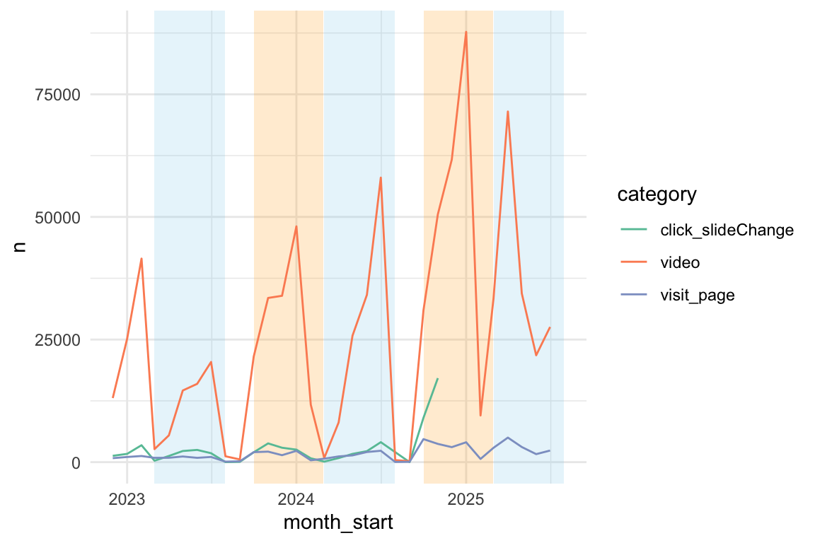
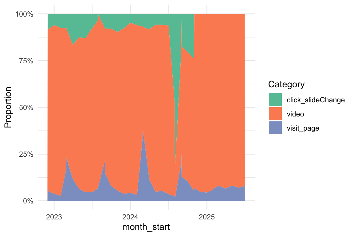
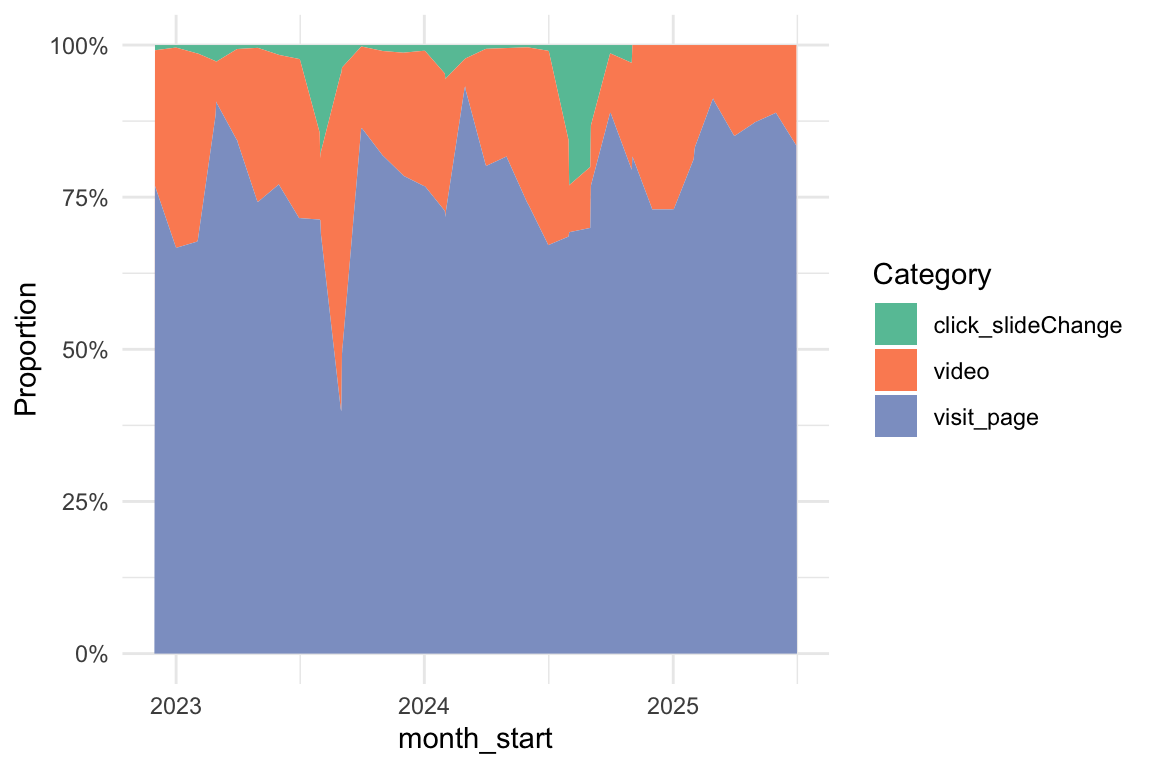
5.2.3.1.2 Relative Anteile
Show the code
n_action_type_per_month_top3 |>
  ggplot(aes(
    x = month_start,
    y = n,
    fill = category # Changed from 'color' to 'fill'
  )) +
  # Use geom_area() and set position="fill" to stack and normalize to 100%
  geom_area(position = "fill") +

  # Optional: Customize the y-axis to show percentages
  scale_y_continuous(labels = scales::label_percent()) +

  labs(
    y = "Proportion",
    fill = "Category"
  )
5.2.3.2 fingerprint unique
5.2.3.2.1 Absolutzahlen
Show the code
time_visit_wday_fingerprint |>
  head(30)
Show the code
n_action_type_per_month_top3_fingerprint <-
  n_action_type |>
  select(nr, fingerprint, category) |>
  distinct(fingerprint, .keep_all = TRUE) |>
  ungroup() |>
  filter(category %in% c("video", "click_slideChange", "visit_page")) |>
  left_join(time_visit_wday_fingerprint |> ungroup()) |>
  select(-c(dow, hour, nr)) |>
  drop_na() |>
  mutate(month_start = lubridate::floor_date(date_time, "month")) |>
  count(month_start, category)
Show the code
n_action_type_per_month_top3_fingerprintShow the code
n_action_type_per_month_top3_fingerprint |>
  ggplot(aes(x = month_start, y = n, color = category, group = category)) +
  # --- Highlight March–July (approx 1 Mar to 31 Jul) ---
  annotate(
    "rect",
    xmin = as.Date("2023-03-01"),
    xmax = as.Date("2023-07-31"),
    ymin = -Inf,
    ymax = Inf,
    alpha = 0.2,
    fill = "skyblue"
  ) +

  annotate(
    "rect",
    xmin = as.Date("2024-03-01"),
    xmax = as.Date("2024-07-31"),
    ymin = -Inf,
    ymax = Inf,
    alpha = 0.2,
    fill = "skyblue"
  ) +
  annotate(
    "rect",
    xmin = as.Date("2025-03-01"),
    xmax = as.Date("2025-07-31"),
    ymin = -Inf,
    ymax = Inf,
    alpha = 0.2,
    fill = "skyblue"
  ) +

  # --- Highlight October–February (semester break or 2nd term) ---
  annotate(
    "rect",
    xmin = as.Date("2023-10-01"),
    xmax = as.Date("2024-02-28"),
    ymin = -Inf,
    ymax = Inf,
    alpha = 0.2,
    fill = "orange"
  ) +
  # annotate("rect",
  #          xmin = as.Date("2024-10-01"), xmax = as.Date("2024-02-28"),
  #          ymin = -Inf, ymax = Inf, alpha = 0.2, fill = "orange") +
  annotate(
    "rect",
    xmin = as.Date("2024-10-01"),
    xmax = as.Date("2025-02-28"),
    ymin = -Inf,
    ymax = Inf,
    alpha = 0.2,
    fill = "orange"
  ) +

  geom_line()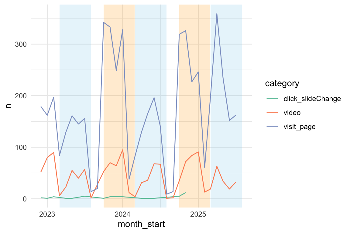
5.2.3.2.2 Relative Anteile
Show the code
n_action_type_per_month_top3_fingerprint |>
  ggplot(aes(
    x = month_start,
    y = n,
    fill = category # Changed from 'color' to 'fill'
  )) +
  # Use geom_area() and set position="fill" to stack and normalize to 100%
  geom_area(position = "fill") +

  # Optional: Customize the y-axis to show percentages
  scale_y_continuous(labels = scales::label_percent()) +

  labs(
    y = "Proportion",
    fill = "Category"
  )
5.2.4 Top3 - Pro Kurs
5.2.4.1 Alle Kurse
Show the code
n_action_type_course_uni <-
  n_action_type |>
  left_join(course_and_uni_per_visit |> mutate(idvisit = as.integer(idvisit)))
Show the code
n_action_type_per_month_top3_per_course |>
  ggplot(aes(x = month_start, y = n, color = category, group = category)) +
  facet_wrap(~course, ncol = 3, scales = "free_y") +
  # --- Highlight March–July (approx 1 Mar to 31 Jul) ---
  annotate(
    "rect",
    xmin = as.Date("2023-03-01"),
    xmax = as.Date("2023-07-31"),
    ymin = -Inf,
    ymax = Inf,
    alpha = 0.2,
    fill = "skyblue"
  ) +

  annotate(
    "rect",
    xmin = as.Date("2024-03-01"),
    xmax = as.Date("2024-07-31"),
    ymin = -Inf,
    ymax = Inf,
    alpha = 0.2,
    fill = "skyblue"
  ) +
  annotate(
    "rect",
    xmin = as.Date("2025-03-01"),
    xmax = as.Date("2025-07-31"),
    ymin = -Inf,
    ymax = Inf,
    alpha = 0.2,
    fill = "skyblue"
  ) +

  # --- Highlight October–February (semester break or 2nd term) ---
  annotate(
    "rect",
    xmin = as.Date("2023-10-01"),
    xmax = as.Date("2024-02-28"),
    ymin = -Inf,
    ymax = Inf,
    alpha = 0.2,
    fill = "orange"
  ) +
  # annotate("rect",
  #          xmin = as.Date("2024-10-01"), xmax = as.Date("2024-02-28"),
  #          ymin = -Inf, ymax = Inf, alpha = 0.2, fill = "orange") +
  annotate(
    "rect",
    xmin = as.Date("2024-10-01"),
    xmax = as.Date("2025-02-28"),
    ymin = -Inf,
    ymax = Inf,
    alpha = 0.2,
    fill = "orange"
  ) +
  geom_line() +
  theme(legend.position = "bottom") +
  scale_x_date(date_labels = "%b %Y")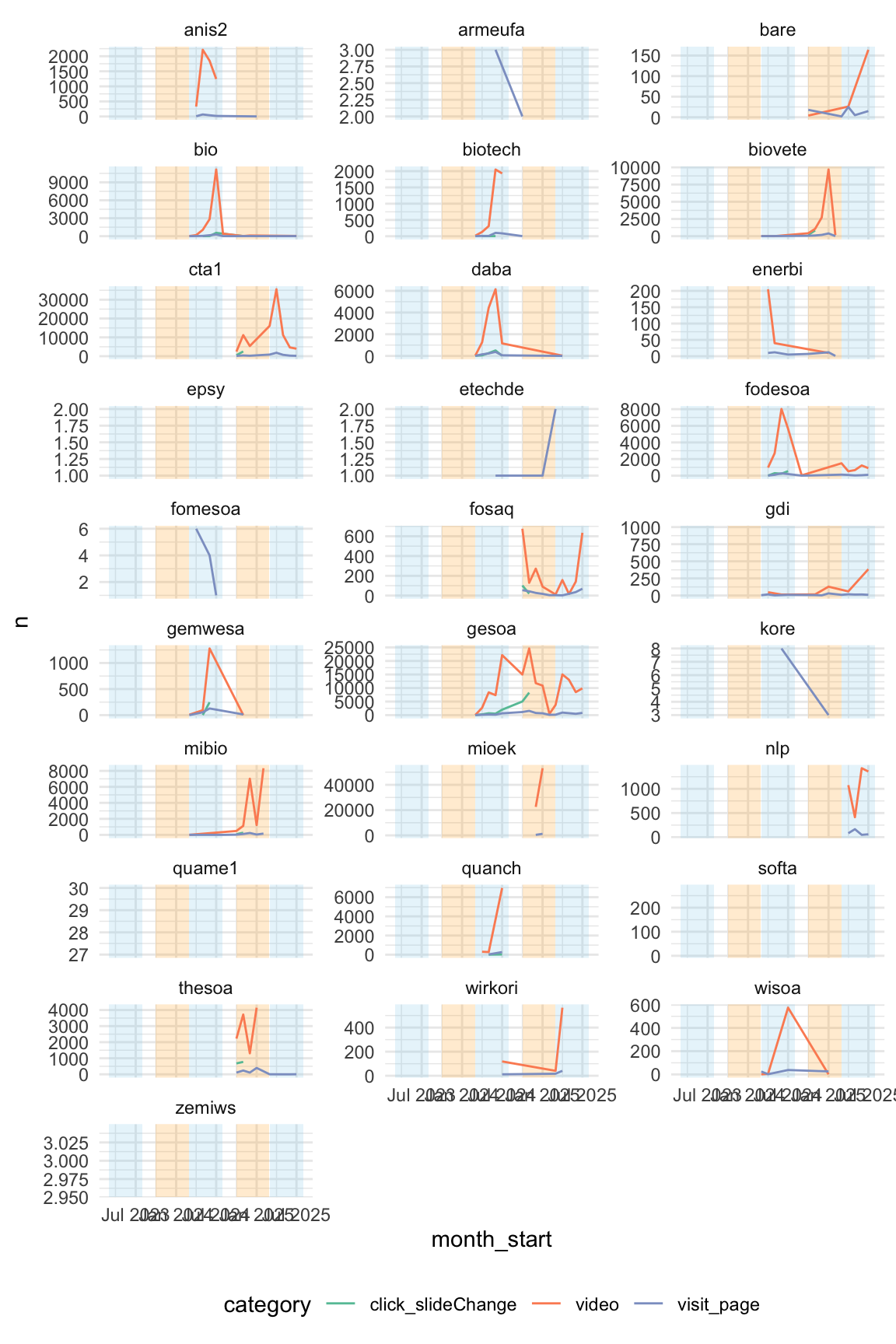
5.2.4.2 CTA1 und GESOA
Show the code
n_action_type_per_month_top3_per_course |>
  filter(course %in% c("cta1", "gesoa")) |>
  ggplot(aes(x = month_start, y = n, color = category, group = category)) +
  # --- Highlight March–July (approx 1 Mar to 31 Jul) ---
  annotate(
    "rect",
    xmin = as.Date("2023-03-01"),
    xmax = as.Date("2023-07-31"),
    ymin = -Inf,
    ymax = Inf,
    alpha = 0.2,
    fill = "skyblue"
  ) +

  annotate(
    "rect",
    xmin = as.Date("2024-03-01"),
    xmax = as.Date("2024-07-31"),
    ymin = -Inf,
    ymax = Inf,
    alpha = 0.2,
    fill = "skyblue"
  ) +
  annotate(
    "rect",
    xmin = as.Date("2025-03-01"),
    xmax = as.Date("2025-07-31"),
    ymin = -Inf,
    ymax = Inf,
    alpha = 0.2,
    fill = "skyblue"
  ) +

  # --- Highlight October–February (semester break or 2nd term) ---
  annotate(
    "rect",
    xmin = as.Date("2023-10-01"),
    xmax = as.Date("2024-02-28"),
    ymin = -Inf,
    ymax = Inf,
    alpha = 0.2,
    fill = "orange"
  ) +
  # annotate("rect",
  #          xmin = as.Date("2024-10-01"), xmax = as.Date("2024-02-28"),
  #          ymin = -Inf, ymax = Inf, alpha = 0.2, fill = "orange") +
  annotate(
    "rect",
    xmin = as.Date("2024-10-01"),
    xmax = as.Date("2025-02-28"),
    ymin = -Inf,
    ymax = Inf,
    alpha = 0.2,
    fill = "orange"
  ) +
  facet_wrap(~course, ncol = 3, scales = "free_y") +
  geom_line() +
  theme(legend.position = "bottom") +
  scale_x_date(date_labels = "%b %Y")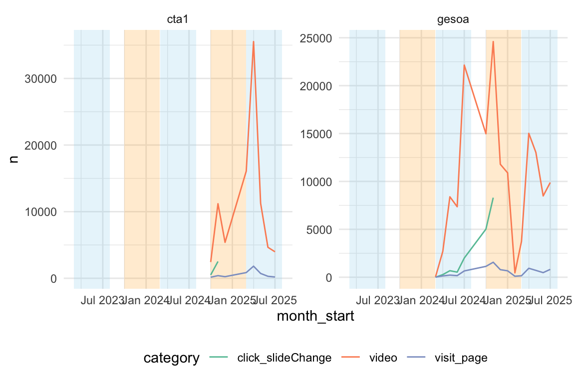
Show the code
n_action_type_per_month_top3_per_course |>
  filter(course %in% c("cta1", "gesoa")) |>
  ggplot(aes(x = month_start, y = n, fill = category, group = category)) +
  facet_wrap(~course, ncol = 3, scales = "free_y") +
  geom_area(position = "fill") +
  theme(legend.position = "bottom") +
  scale_x_date(date_labels = "%b %Y") +
scale_y_continuous(labels = scales::label_percent()) 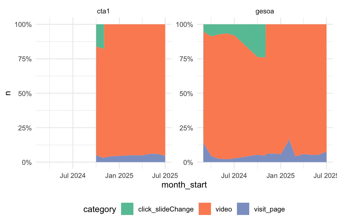
5.2.5 eventcategory
5.2.5.1 Insgesamt
Für folgende Analyse wurde eine andere Variable als oben herangezogen, nämlich eventcategory. Dadurch resultieren etwas andere Ergebnisse - ausführlichere.
Show the code
data_eventcategory <-
  data_separated_filtered |>
  filter(type == "eventcategory")
Show the code
Show the code
data_separated_filtered_count |>
  ggtexttable()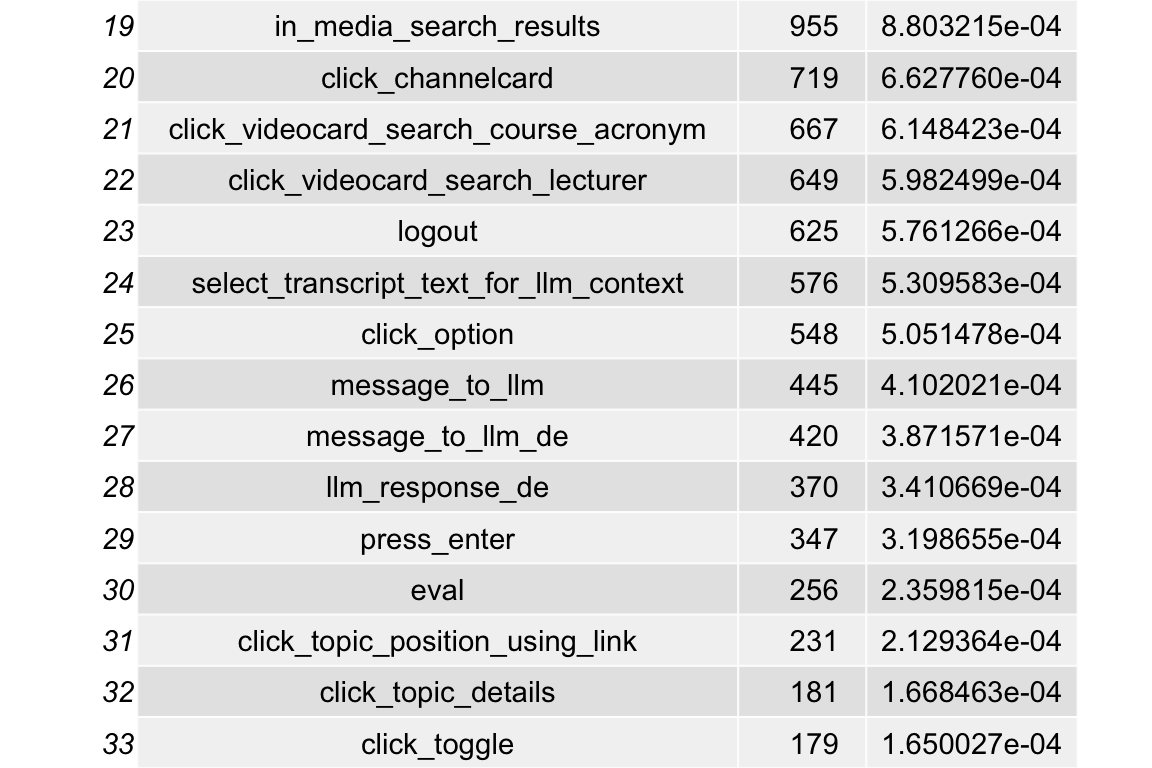
Show the code
#data_separated_filtered_count |>
#  writexl::write_xlsx(path = "obj/data_separated_filtered_count.xlsx")
5.2.5.2 Pro Universität
Sortiert nach Häufigkeiten pro Hochschule
Show the code
data_separated_filtered_date_uni_course_top5_uni <-
  data_separated_filtered_date_uni_course |>
  compute_prop_eventcategory_per_uni_course()

data_separated_filtered_date_uni_course_top5_uni |>
kable(digits = 2)| university | value | n | total_n | prop |
|---|---|---|---|---|
| evhn | videoplayer_click | 696 | 798 | 0.87 |
| evhn | click_slideChange | 29 | 798 | 0.04 |
| evhn | click_videocard | 18 | 798 | 0.02 |
| evhn | select_transcript_text_for_llm_context | 12 | 798 | 0.02 |
| evhn | click_button | 8 | 798 | 0.01 |
| hnu | videoplayer_click | 182 | 358 | 0.51 |
| hnu | verify_option_wrong | 48 | 358 | 0.13 |
| hnu | click_button | 31 | 358 | 0.09 |
| hnu | static_questionaire | 14 | 358 | 0.04 |
| hnu | static_questionaire_difficulty | 14 | 358 | 0.04 |
| hs-ansbach | videoplayer_click | 27 | 59 | 0.46 |
| hs-ansbach | click_button | 16 | 59 | 0.27 |
| hs-ansbach | click_channelcard_search_course_acronym | 3 | 59 | 0.05 |
| hs-ansbach | click_transcript_word | 3 | 59 | 0.05 |
| hs-ansbach | click_videocard | 3 | 59 | 0.05 |
| hswt | videoplayer_click | 89318 | 99330 | 0.90 |
| hswt | click_button | 3403 | 99330 | 0.03 |
| hswt | click_slideChange | 3018 | 99330 | 0.03 |
| hswt | click_videocard | 904 | 99330 | 0.01 |
| hswt | login | 685 | 99330 | 0.01 |
| iqw | videoplayer_click | 8 | 21 | 0.38 |
| iqw | click_button | 4 | 21 | 0.19 |
| iqw | click_channelcard | 2 | 21 | 0.10 |
| iqw | in_media_search | 2 | 21 | 0.10 |
| iqw | in_media_search_results | 2 | 21 | 0.10 |
| th-nuernberg | videoplayer_click | 270771 | 376939 | 0.72 |
| th-nuernberg | clear_transcript_text_for_llm_context | 60995 | 376939 | 0.16 |
| th-nuernberg | click_slideChange | 23573 | 376939 | 0.06 |
| th-nuernberg | click_button | 4655 | 376939 | 0.01 |
| th-nuernberg | click_videocard | 3038 | 376939 | 0.01 |
| th-owl | videoplayer_click | 3 | 4 | 0.75 |
| th-owl | click_mediaitem | 1 | 4 | 0.25 |
| thi | videoplayer_click | 75079 | 77182 | 0.97 |
| thi | click_button | 632 | 77182 | 0.01 |
| thi | click_videocard | 495 | 77182 | 0.01 |
| thi | click_transcript_word | 365 | 77182 | 0.00 |
| thi | login | 228 | 77182 | 0.00 |
Show the code
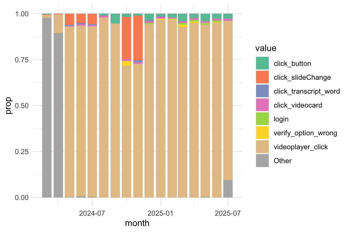
data_separated_filtered_date_uni_course_top5_uni |>
  # --- Visualization ---
  ggplot(aes(
    x = reorder(value, prop), # Reorder bars by proportion within each facet
    y = prop,
    fill = value # Use 'value' for color
  )) +

  # Bar chart
  geom_col() +

  # Separate plot for each university
  facet_wrap(~university, scales = "free_y", ncol = 1) +

  # Flip coordinates for better readability of long category names
  coord_flip() +

  # Clean up labels and aesthetics
  scale_y_continuous(labels = label_percent()) +
  labs(
    title = "Top 5 'eventcategory' Values by University",
    subtitle = "Proportion of total events within each university",
    x = "Event Category (Value)",
    y = "Proportion (%)",
    fill = "Category"
  ) +
  # Use a minimal theme
  theme_minimal() +
  # Remove the legend since the categories are on the y-axis
  theme(legend.position = "none")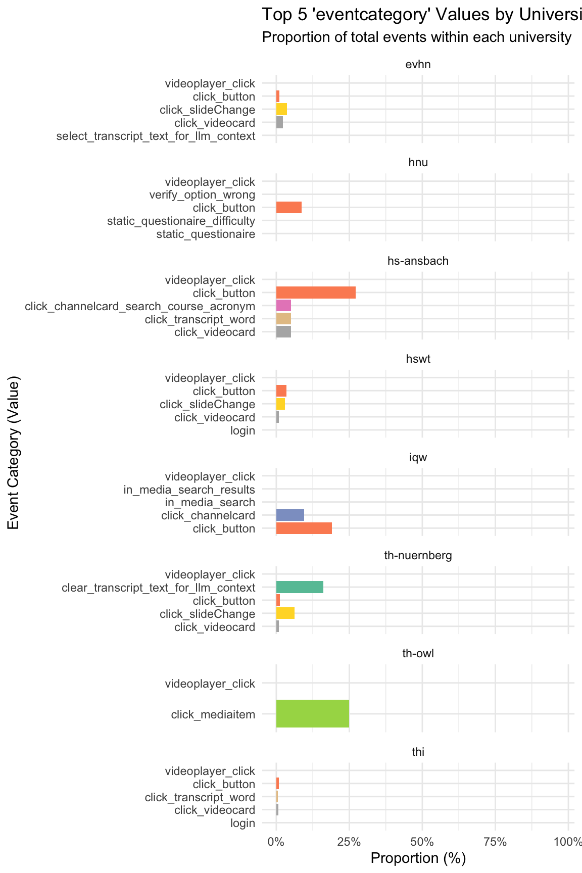
Show the code
data_separated_filtered_date_uni_course_top5_uni |>
  ungroup() |>
  mutate(value = fct_lump(value, 5)) |>
  ggplot(aes(x = university, y = n, fill = value)) +
  geom_col(position = "fill") +

  # Ensure the Y-axis range is correct
  scale_y_continuous(
    labels = scales::label_percent()
  ) +

  labs(
    title = "Top 5 Event Category Proportions by University",
    y = "Proportion of Total Events (%)",
    x = "University",
    fill = "Event Category"
  ) +
  theme_minimal()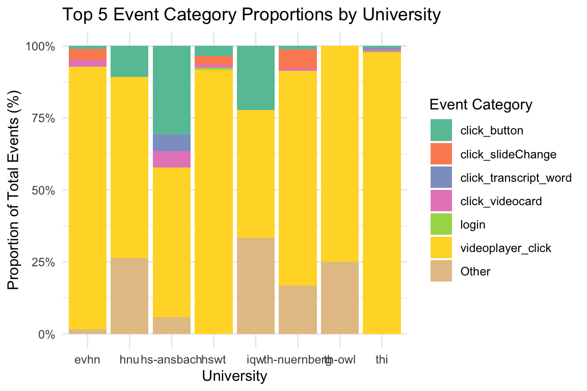
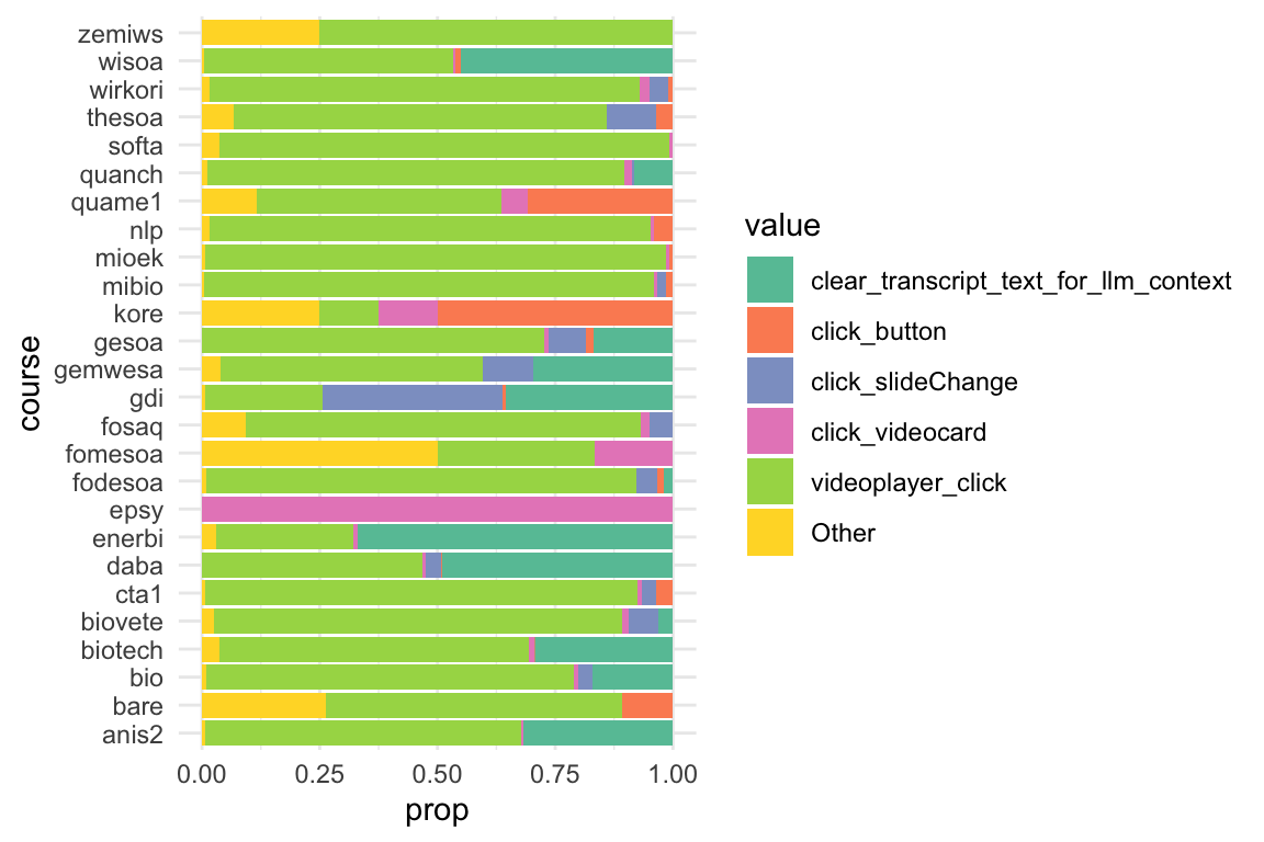
5.2.5.3 Pro Kurs
Show the code
data_separated_filtered_date_uni_course_top5_course <-
  data_separated_filtered_date_uni_course |>
  compute_prop_eventcategory_per_uni_course(group_var = course)
Show the code
5.2.5.4 Jahr
Show the code
data_separated_filtered_date_uni_course_top5_date <-
  data_separated_filtered_date_uni_course |>
  compute_prop_eventcategory_per_uni_course(group_var = month)
Show the code
Show the code
data_separated_filtered_date_uni_course_top5_date |>

  mutate(value = fct_lump(value, 5)) |>
  # 2. Visualization
  ggplot(aes(
    x = month,
    y = prop, # Plot the calculated proportion
    fill = value # Use 'value' for the fill (stacking segments)
  )) +

  # Use geom_area() with position = "fill" to ensure the areas stack to 100%
  geom_area(position = "fill") +

  # Customize the Y-axis to show percentages
  scale_y_continuous(labels = scales::label_percent()) +

  # Customize the X-axis for dates
  scale_x_datetime(
    breaks = pretty_breaks(n = 6), # Request roughly 6 "nice" breaks
    date_labels = "%b %Y" # Label format: e.g., "Mar 2024"
  ) +
  # Labels and Theme
  labs(
    title = "Relative Frequency of Top Event Categories Over Time",
    subtitle = "Showing the monthly composition of the top 5 events",
    x = "Month",
    y = "Proportion of Total Events (%)",
    fill = "Event Category"
  ) +
  theme_minimal() +
  theme(axis.text.x = element_text(angle = 45, hjust = 1))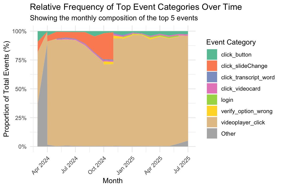
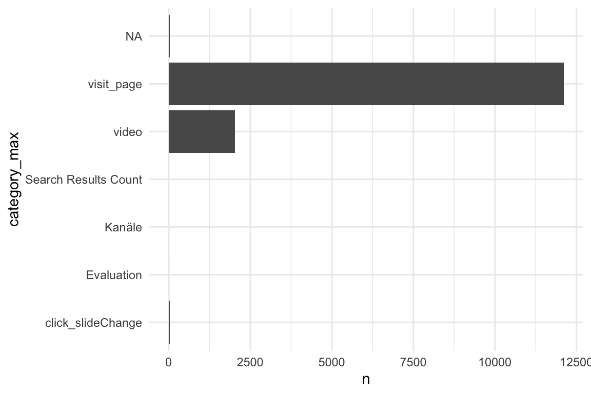
5.2.6 User-Typen nach Aktivitäten
Was ist die Hauptaktivität pro User? - Verteilung
5.2.6.1 idvisit
Show the code
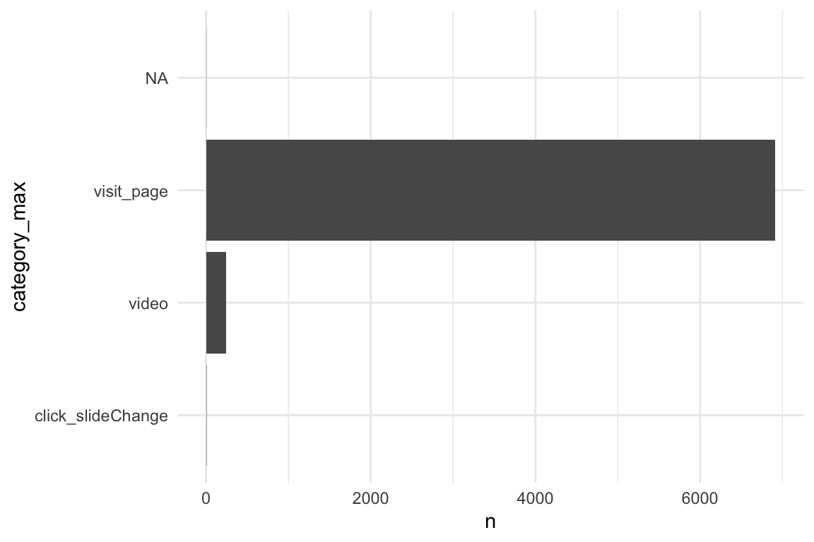
5.2.6.2 fingerprint
Show the code
5.3 Verteilung der Nutzer-Aktionen
Show the code
n_action_type_counted <-
  n_action_type |>
  count(category, sort = TRUE)
5.3.1 Insgesamt - Rohwerte
Show the code
n_action_type_counted |>
  ggplot(aes(y = reorder(category, n), x = n)) +
  geom_col() +
  geom_bar_text() +
  labs(
    x = "User-Aktion",
    y = "Aktion",
    title = "Anzahl der User-Aktionen nach Kategorie"
  ) +
  theme_minimal() +
  scale_x_continuous(labels = scales::comma)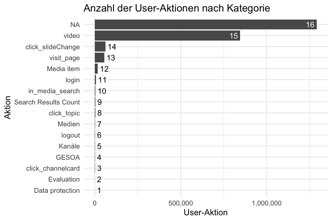
5.3.2 Insgesamt - Log-Skalierung
Show the code
n_action_type_counted |>
  ggplot(aes(y = reorder(category, n), x = n)) +
  geom_col() +
  geom_bar_text() +
  labs(
    x = "Anzahl der User-Aktionen",
    y = "Aktion",
    title = "Anzahl der User-Aktionen nach Kategorie",
    caption = "Log10-Skala"
  ) +
  theme_minimal() +
  scale_x_log10()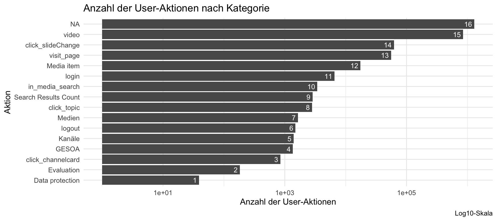
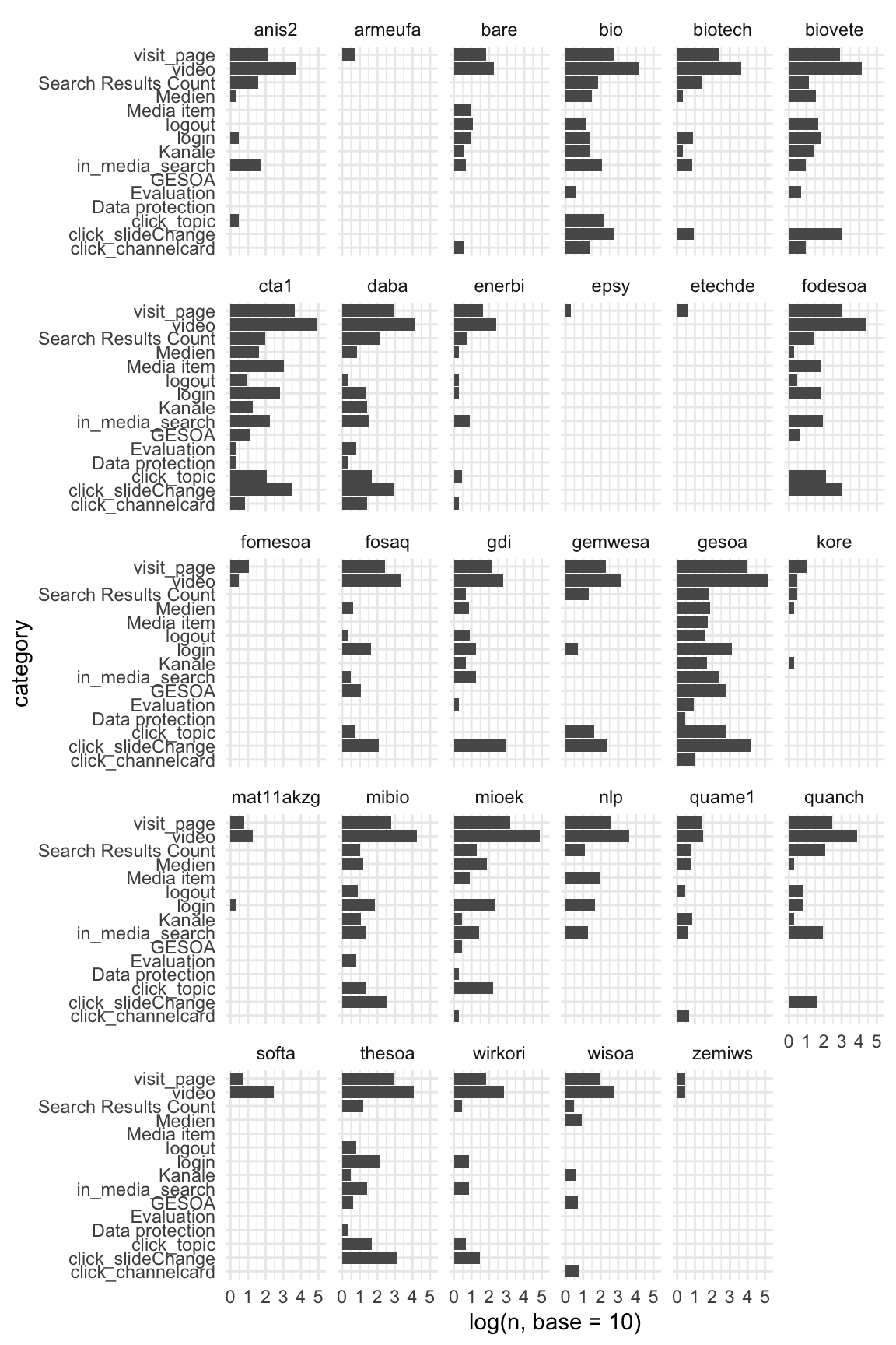
5.3.3 Pro Kurs - Rohwerte
Show the code
n_action_type_course_uni_counted |>
  ggplot() +
  aes(y = category, x = log(n, base = 10)) +
  geom_col() +
  facet_wrap(~course)