4 Verweildauer pro Visit
4.1 Setup
Show the code
source("_common.r")4.2 Berechnungsgrundlage der Verweildauer
Die Verweildauer wurde berechnet als Differenz zwischen kleinstem und größtem Datumszeitwert (POSixct) eines Visits (also pro Wert der Variablen idvisit), vgl. Funktion diff_time. Diese Variable heißt time_diff im Objekt time_spent.
Dabei wird das Objekt data_separated_filtered herangezogen, vgl. die Definition es Targets “time_spent” in der Targets-Pipeline.
4.3 Vorverarbeitung
Die Visit-Zeit wurde auf 600 Min. trunkiert/begrenzt.
4.3.1 idvisit
Show the code
time_spent |>
  head(30)
Show the code
time_spent <-
  time_spent |>
  # compute time (t) in minutes (min):
  mutate(t_minutes = as.numeric(time_diff, units = "mins")) |>
  filter(t_minutes < 600)
4.3.2 fingerprint
Show the code
time_spent_fingerprint |>
  head(30)
Show the code
time_spent_fingerprint <-
  time_spent_fingerprint |>
  # compute time (t) in minutes (min):
  mutate(t_minutes = as.numeric(time_diff, units = "mins")) |>
  filter(t_minutes < 600)
4.3.3 fingerprint unqiue
Show the code
time_spent_fingerprint |>
  head(30)
Show the code
time_spent_fingerprint_unique <-
  time_spent_fingerprint |>
  distinct(fingerprint, .keep_all = TRUE) |>
  # compute time (t) in minutes (min):
  mutate(t_minutes = as.numeric(time_diff, units = "mins")) |>
  filter(t_minutes < 600)
4.4 Verweildauer-Statistiken in Sekunden
Die Verweildauer ist im Folgenden dargestellt auf Grundlage oben dargestellter Berechnungsgrundlage (in Sekunden).
4.4.1 idvisit
4.4.2 fingerprint
4.4.3 fingerprint unqiue
4.5 Verweildauer auf Basis der Variable visitduration
4.5.1 Für alle Daten
Alternativ zur Berechnung der Verweildauer steht eine Variable, visitduration zur Verfügung, die (offenbar) die Dauer des Visits misst bzw. messen soll.
Allerdings resultieren substanziell andere Werte, wenn man diese Variable heranzieht zur Berechnung der Verweildauer, vgl. Target time_duration in der Targets-Pipeline.
Show the code
time_duration |>
head(30)4.5.2 Für unique idvisits
4.5.3 Für unique fingerprints
4.6 Verweildauer-Statistiken in Minuten
Show the code
time_spent_summary <-
time_spent |>
  mutate(time_diff_minutes = time_length(time_diff, unit = "minute")) |>
  summarise(
    mean_time_diff = round(mean(time_diff_minutes), 2),
    sd_time_diff = sd(time_diff_minutes),
    min_time_diff = min(time_diff_minutes), # shortest duration
    max_time_diff = max(time_diff_minutes) # longest
  )

time_spent_summary |>
gt()| mean_time_diff | sd_time_diff | min_time_diff | max_time_diff |
|---|---|---|---|
| 29.86 | 39.92699 | 0 | 476.15 |
Show the code
small_padding_theme <- ggpubr::ttheme(
  tbody.style = tbody_style(size = 8), # Smaller font size can help
  colnames.style = colnames_style(size = 9, face = "bold"),
  padding = unit(c(2, 2), "mm") # Reduce horizontal and vertical padding
)
Show the code
ggpubr::ggtexttable(
  time_spent_summary,
  rows = NULL,
  theme = small_padding_theme
)
4.7 Visualisierung der Verweildauer
4.7.1 Binwidth=10 Minutes
Show the code
time_spent |>
  mutate(time_diff_minutes = time_diff / 60) |>
  ggplot(aes(x = time_diff_minutes)) + # minutes
  geom_histogram(binwidth = 10) +
  #scale_x_time() +
  theme_minimal() +
  labs(y = "n", x = "Verweildauer in HaNS pro Visit in d:h:m") +
  scale_x_time(breaks = pretty_breaks()) +
  geom_vline(xintercept = median(time_spent$time_diff) / 60, color = "blue", linetype = "dashed") +
  annotate("label", x = median(time_spent$time_diff) / 60,
           y = Inf, label = "Median", vjust = 1.5, color = "blue")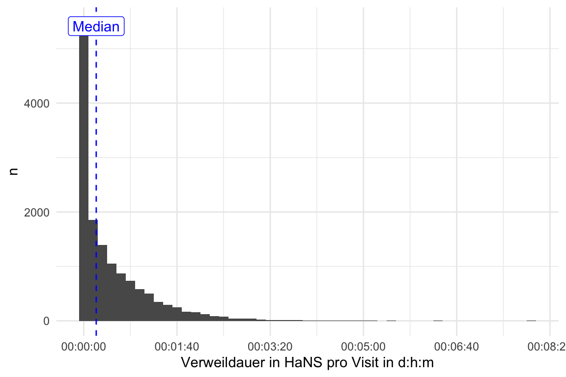
4.7.2 Bin width= 20 Minutes
Show the code
time_spent |>
  mutate(time_diff_minutes = time_diff / 60) |>
  ggplot(aes(x = time_diff_minutes)) + # minutes
  geom_histogram(binwidth = 20) +
  theme_minimal() +
  labs(
    y = "n",
    x = "Verweildauer",
    title = "Verweildauer in HaNS pro Visit in d:h:m"
  ) +
  scale_x_time(breaks = pretty_breaks()) +
  annotate("label", x = median(time_spent$time_diff) / 60,
           y = Inf, label = "Median", vjust = 1.5, color = "blue")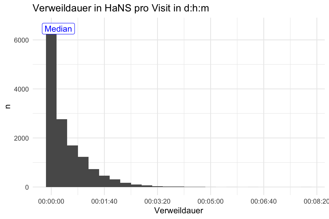
4.7.3 Zeitdauer begrenzt auf 1-120 Min.
Show the code
time_spent2 <-
  time_spent |>
  filter(time_diff > 1, time_diff < 120)

time_spent2 |>
  ggplot(aes(x = time_diff)) +
  geom_histogram(binwidth = 10) +
  theme_minimal() +
  labs(
    y = "n",
    x = "Verweildauer in HaNS pro Visit in Minuten",
    title = "Verweildauer begrenzt auf 1-120 Minuten",
    caption = "bindwidth = 10 Min."
  ) +
  annotate("label", x = median(time_spent$time_diff) / 60,
           y = Inf, label = "Median", vjust = 1.5, color = "blue")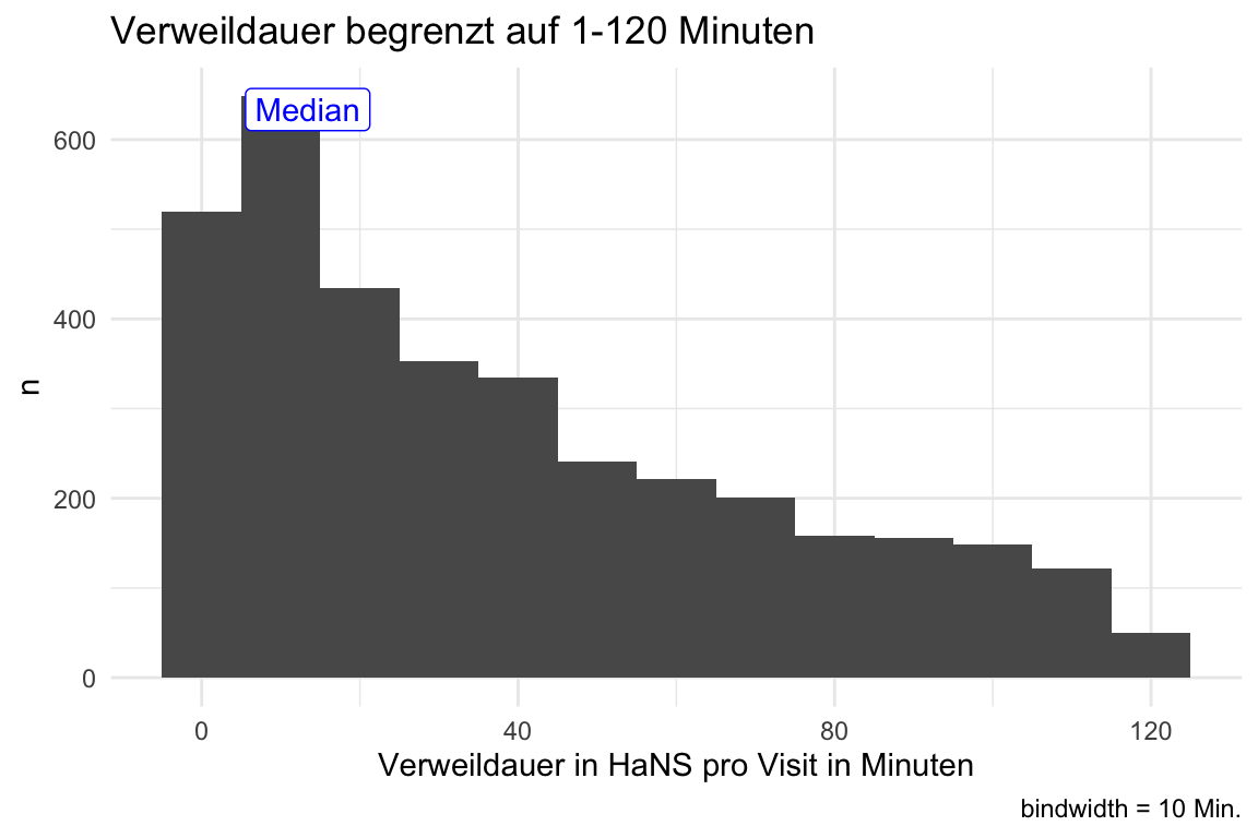
4.7.4 Veränderung der Verweildauer im Zeitverlauf
4.7.4.1 Monat
Die Einheit von time_spent ist Sekunden.
Show the code
time_spent_by_month <-
  time_spent |>
  mutate(month_start = floor_date(time_min, "month")) |>
  mutate(
    month_name = lubridate::month(month_start, label = TRUE, abbr = FALSE),
    month_num = lubridate::month(month_start, label = FALSE),
    year = lubridate::year(month_start)
  ) |>
  group_by(month_num, year) |>
  summarise(
    time_spent_month_avg = mean(time_diff, na.rm = TRUE),
    time_spent_month_sd = sd(time_diff, na.rm = TRUE)
  ) |>
  arrange(year, month_num)

time_spent_by_month
Show the code
time_spent_by_month |>
  mutate(
    time_spent_month_avg = round(time_spent_month_avg, 2),
    time_spent_month_sd = round(time_spent_month_sd, 2)
  ) |>
  ggtexttable()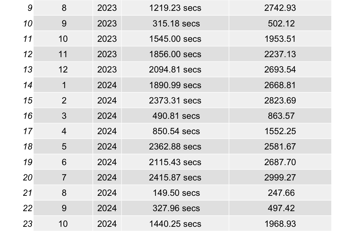
Show the code
time_spent_by_month_name <-
  time_spent |>
  mutate(month_start = lubridate::floor_date(time_min, "month")) |>
  mutate(
    month_name = lubridate::month(month_start, label = TRUE, abbr = FALSE),
    month_num = lubridate::month(month_start, label = FALSE),
    year = lubridate::year(month_start)
  ) |>
  group_by(month_start, year) |>
  summarise(
    time_spent_month_avg = mean(time_diff, na.rm = TRUE),
    time_spent_month_sd = sd(time_diff, na.rm = TRUE)
  )

time_spent_by_month_name |>
  ggplot(aes(x = month_start, y = time_spent_month_avg)) +
  geom_line(group = 1, color = "grey60") +
  scale_y_time(labels = scales::time_format("%H:%M:%S")) +
  labs(x = "Datum", y = "Durchschnittliche Verweildauer pro Visit (in h:m:s)") +
  # --- Highlight March–July (approx 1 Mar to 31 Jul) ---
  annotate(
    "rect",
    xmin = as.Date("2023-03-01"),
    xmax = as.Date("2023-07-31"),
    ymin = -Inf,
    ymax = Inf,
    alpha = 0.2,
    fill = "skyblue"
  ) +

  annotate(
    "rect",
    xmin = as.Date("2024-03-01"),
    xmax = as.Date("2024-07-31"),
    ymin = -Inf,
    ymax = Inf,
    alpha = 0.2,
    fill = "skyblue"
  ) +
  annotate(
    "rect",
    xmin = as.Date("2025-03-01"),
    xmax = as.Date("2025-07-31"),
    ymin = -Inf,
    ymax = Inf,
    alpha = 0.2,
    fill = "skyblue"
  ) +

  # --- Highlight October–February (semester break or 2nd term) ---
  annotate(
    "rect",
    xmin = as.Date("2023-10-01"),
    xmax = as.Date("2024-02-28"),
    ymin = -Inf,
    ymax = Inf,
    alpha = 0.2,
    fill = "orange"
  ) +
  # annotate("rect",
  #          xmin = as.Date("2024-10-01"), xmax = as.Date("2024-02-28"),
  #          ymin = -Inf, ymax = Inf, alpha = 0.2, fill = "orange") +
  annotate(
    "rect",
    xmin = as.Date("2024-10-01"),
    xmax = as.Date("2025-02-28"),
    ymin = -Inf,
    ymax = Inf,
    alpha = 0.2,
    fill = "orange"
  ) +

  geom_point()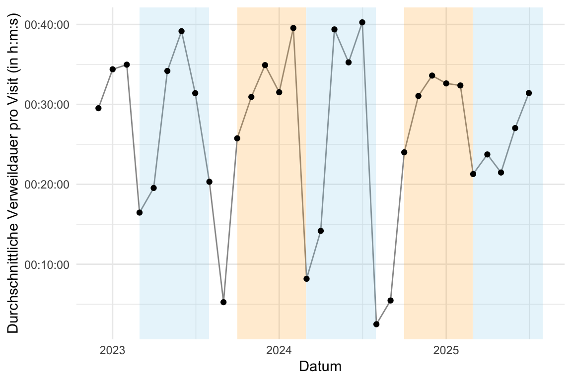
4.7.4.2 Jahr
Show the code
time_spent_by_year <-
  time_spent |>
  mutate(month_start = lubridate::floor_date(time_min, "month")) |>
  mutate(
    month_name = lubridate::month(month_start, label = TRUE, abbr = FALSE),
    month_num = lubridate::month(month_start, label = FALSE),
    year = year(month_start)
  ) |>
  group_by(year) |>
  summarise(
    time_spent_avg = mean(time_diff, na.rm = TRUE),
    time_spent_sd = sd(time_diff, na.rm = TRUE)
  )

time_spent_by_year
Show the code
time_spent_by_year <-
  time_spent_by_year |>
  mutate(year_date = lubridate::ymd(paste0(year, "-01-01"))) # MAKE Date class

rect_data <- comp_semester_rects(time_spent_by_year, col_date = "year_date")

time_spent_by_year |>
  ggplot(aes(x = year_date, y = time_spent_avg)) +
  scale_x_date(date_labels = "%Y") +
  geom_line(group = 1, color = "grey60") +
  geom_rect(
    data = rect_data |> mutate(xmin = as.Date(xmin), xmax = as.Date(xmax)), # ensure Date
    aes(xmin = xmin, xmax = xmax, ymin = ymin, ymax = ymax),
    fill = "grey",
    alpha = 0.2,
    inherit.aes = FALSE
  ) +
  geom_point() +
  scale_y_time(labels = scales::time_format("%H:%M")) +
  labs(x = "Jahr", y = "Durchschnittliche Verweildauer pro Jahr (h:m)")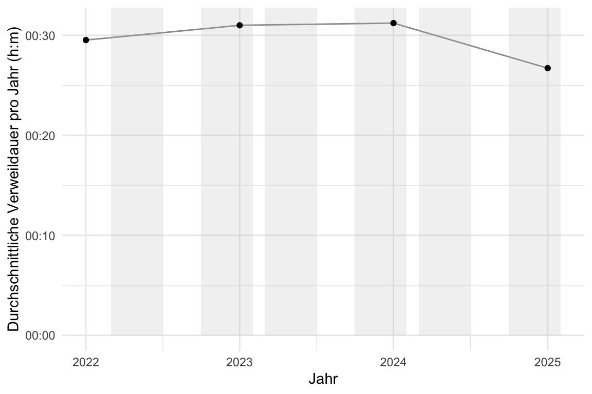
Show the code
# ...existing code...4.7.4.3 Woche
Show the code
time_spent_by_week_name <-
  time_spent |>
  mutate(week_start = lubridate::floor_date(time_min, "week")) |>
  mutate(week_num = lubridate::week(week_start), year = year(week_start)) |>
  group_by(week_start, year) |>
  summarise(
    time_spent_week_avg = mean(time_diff, na.rm = TRUE),
    time_spent_week_sd = sd(time_diff, na.rm = TRUE)
  )

time_spent_by_week_name |>
  ggplot(aes(x = week_start, y = time_spent_week_avg)) +
  scale_y_time(labels = scales::time_format("%H:%M")) +
  labs(x = "Datum", y = "Durchschnittliche Verweildauer pro Woche (h:m)") +

  # --- Highlight March–July (approx 1 Mar to 31 Jul) ---
  annotate(
    "rect",
    xmin = as.Date("2023-03-01"),
    xmax = as.Date("2023-07-31"),
    ymin = -Inf,
    ymax = Inf,
    alpha = 0.2,
    fill = "skyblue"
  ) +

  annotate(
    "rect",
    xmin = as.Date("2024-03-01"),
    xmax = as.Date("2024-07-31"),
    ymin = -Inf,
    ymax = Inf,

    alpha = 0.2,
    fill = "skyblue"
  ) +
  annotate(
    "rect",
    xmin = as.Date("2025-03-01"),
    xmax = as.Date("2025-07-31"),
    ymin = -Inf,
    ymax = Inf,
    alpha = 0.2,
    fill = "skyblue"
  ) +

  # --- Highlight October–February (semester break or 2nd term) ---
  annotate(
    "rect",
    xmin = as.Date("2023-10-01"),
    xmax = as.Date("2024-02-28"),
    ymin = -Inf,
    ymax = Inf,
    alpha = 0.2,
    fill = "orange"
  ) +
  # annotate("rect",
  #          xmin = as.Date("2024-10-01"), xmax = as.Date("2024-02-28"),
  #          ymin = -Inf, ymax = Inf, alpha = 0.2, fill = "orange") +
  annotate(
    "rect",
    xmin = as.Date("2024-10-01"),
    xmax = as.Date("2025-02-28"),
    ymin = -Inf,
    ymax = Inf,
    alpha = 0.2,
    fill = "orange"
  ) +
  geom_line(group = 1, color = "grey60") +
  geom_point() +
  geom_smooth(method = "loess", se = FALSE, color = "blue")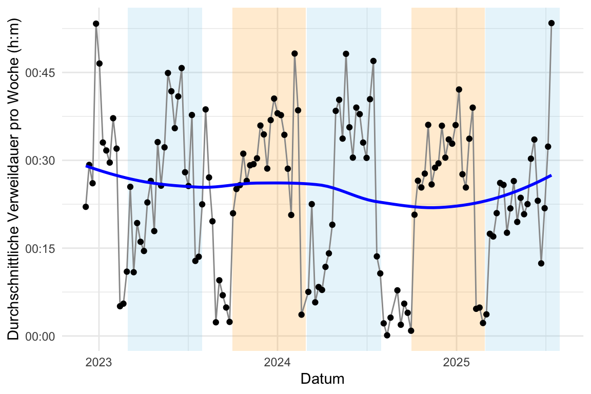
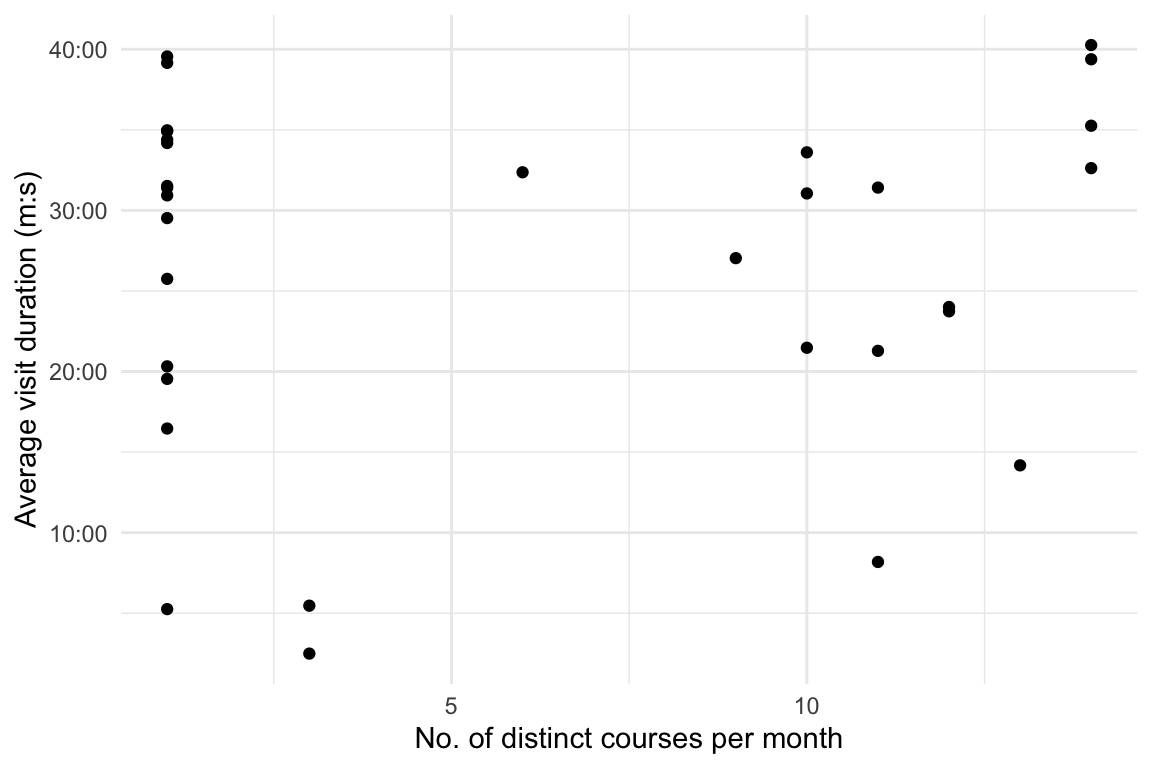
4.8 Zusammenhang von Lehrveranstaltung und Verweildauer
Show the code
time_spent_w_course_university_summary <-
  time_spent_w_course_university |>
  group_by(floor_date_month) |>
  summarise(
    distinct_courses_n = n_distinct(course),
    diff_time_mean = mean(time_diff, na.rm = TRUE),
    n = n()
  )

time_spent_w_course_university_summary
Show the code
time_spent_w_course_university_summary |>
  ggplot(aes(x = distinct_courses_n, y = diff_time_mean)) +
  geom_point() +
  scale_y_time(labels = scales::time_format("%M:%S")) +
  labs(
    y = "Average visit duration (m:s)",
    x = "No. of distinct courses per month"
  )
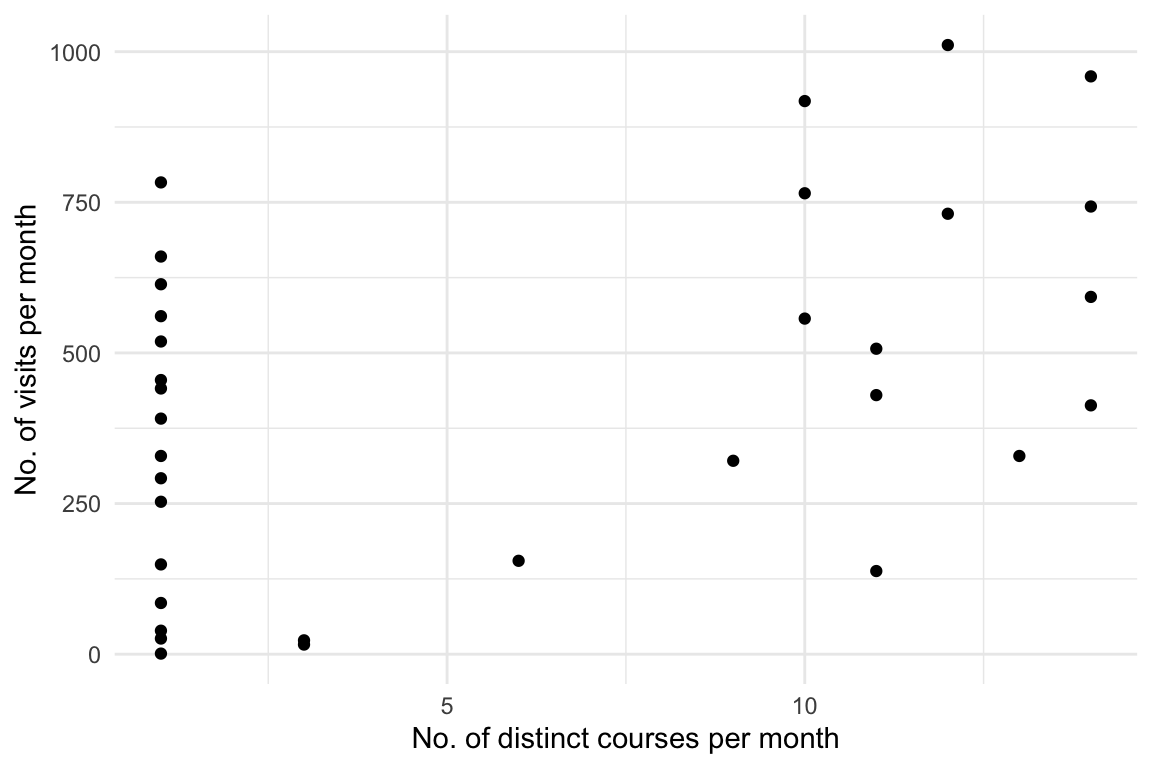
4.9 Zusammenhang von Lehrveranstaltung und Anzahl Visits
Show the code
time_spent_w_course_university_summary |>
  ggplot(aes(x = distinct_courses_n, y = n)) +
  geom_point() +
  labs(y = "No. of visits per month", x = "No. of distinct courses per month")