7 Videonutzung
7.1 Setup
Show the code
source("_common.r")Wie viel Zeit verbringen die Nutzer mit dem Betrachten von Videos (“Glotzdauer”)?
7.2 Glotzdauer allgemein
Achtung: Die Videozeit ist schwierig auszuwerten: Die Nutzer beenden keine Videos, in dem sie auf “Pause” drücken, sondern indem sie andere Aktionen durchführen. Dies ist aber analytisch schwer abzubilden.
Vgl. die Definition des Targets glotzdauer in der Pipeline.
Kurz gesagt wird die Zeit-Differenz zwischen zwei aufeinander folgenden “Play” und “Pause” Aktionen berechnet.
Allerdings hat dieses Vorgehen Schwierigkeiten: Nicht immer folgt auf einem “Play” ein “Pause”. Es ist schwer auszuwerten, wann die Betrachtung eines Videos endet. Daher ist diese Analyse nur vorsichtig zu interpretieren.
Die Definition der Funktion glotzdauer.R ist online dokumentiert.
Show the code
Show the code
data_separated_distinct_slice_summary <-
  data_separated_distinct_slice |>
  mutate(time_diff = abs(time_diff)) |>
  # without glotzdauer smaller than 10 minutes:
  filter(time_diff < 60 * 10) |>
  summarise(
    time_diff_median = median(time_diff, na.rm = TRUE),
    time_diff_median_hms = hms::as_hms(median(time_diff, na.rm = TRUE)),
    time_diff_mean_hms = hms::as_hms(mean(time_diff, na.rm = TRUE)),
    time_diff_mean = mean(time_diff, na.rm = TRUE),
    time_diff_sd = sd(time_diff, na.rm = TRUE),
    n = n()
  )
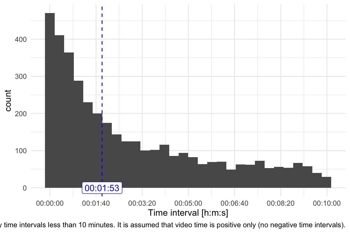
data_separated_distinct_slice_summary |> kable(digits = 2)| time_diff_median | time_diff_median_hms | time_diff_mean_hms | time_diff_mean | time_diff_sd | n |
|---|---|---|---|---|---|
| 113 secs | 00:01:53 | 00:02:54.228375 | 174.23 secs | 167.46 | 3919 |
Für die folgende Darstellung wurden die absoluten Zeitwerte verwendet, d.h. ohne Vorzeichen.
Show the code
data_separated_distinct_slice |>
  # we will assume that negative glotzdauer is the as positive glotzdauer:
  mutate(time_diff = abs(time_diff)) |>
  # without glotzdauer smaller than 10 minutes:
  filter(time_diff < 60 * 10) |>
  ggplot(aes(x = time_diff)) +
  geom_histogram() +
  scale_x_time(breaks = pretty_breaks()) +
  labs(
    x = "Time interval [h:m:s]",
    caption = "Only time intervals less than 10 minutes. It is assumed that video time is positive only (no negative time intervals)."
  ) +
  theme_minimal() +
  geom_vline(xintercept = data_separated_distinct_slice_summary$time_diff_median,
  linetype = "dashed", color = "blue") +
  annotate("label",
    x = data_separated_distinct_slice_summary$time_diff_median_hms,
    y = 0,
    color = "blue",
    label = data_separated_distinct_slice_summary$time_diff_median_hms,
  )
Show the code
| Variable | Mean | SD | IQR | Range | Skewness | Kurtosis | n | n_Missing |
|---|---|---|---|---|---|---|---|---|
| time_diff_abs_sec | 174.23 | 167.46 | 243.00 | (0.00, 599.00) | 0.93 | -0.31 | 3919 | 0 |
| time_diff_abs_min | 2.90 | 2.79 | 4.05 | (0.00, 9.98) | 0.93 | -0.31 | 3919 | 0 |
Show the code
glotzdauer_tbl |>
  mutate(across(where(is.numeric), ~ round(., 2))) |>
  ggpubr::ggtexttable()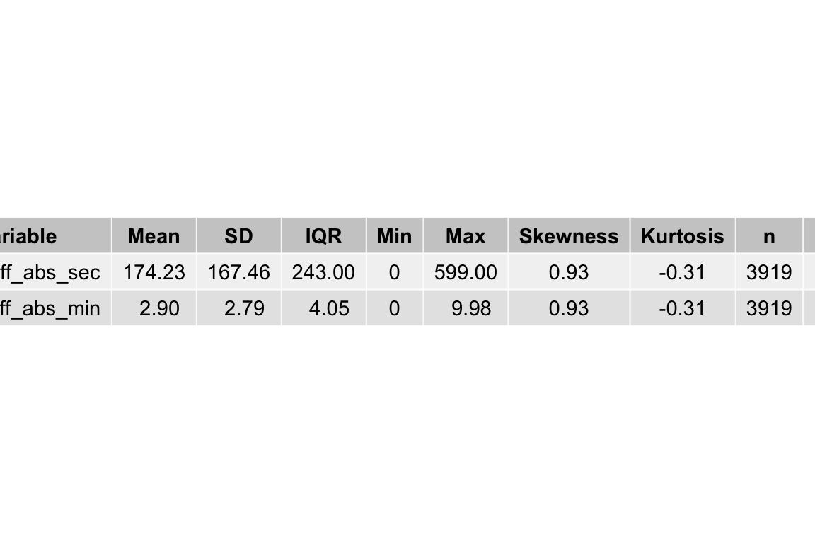
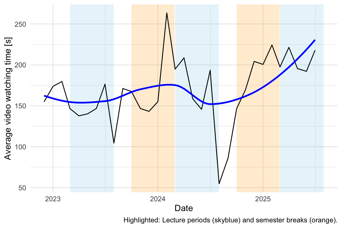
7.3 Glotzdauer im Zeitverlauf
Show the code
glotzdauer_prepped_tbl <-
  glotzdauer_prepped |>
  mutate(first_of_month = floor_date(first_play, unit = "month")) |>
  group_by(first_of_month) |>
  summarise(time_diff_mean = mean(time_diff, na.rm = TRUE))


glotzdauer_prepped_tbl
Show the code
glotzdauer_prepped_tbl |>
  ggplot(aes(x = first_of_month, y = time_diff_mean)) +
  annotate(
    "rect",
    xmin = as.Date("2023-03-01"),
    xmax = as.Date("2023-07-31"),
    ymin = -Inf,
    ymax = Inf,
    alpha = 0.2,
    fill = "skyblue"
  ) +

  annotate(
    "rect",
    xmin = as.Date("2024-03-01"),
    xmax = as.Date("2024-07-31"),
    ymin = -Inf,
    ymax = Inf,
    alpha = 0.2,
    fill = "skyblue"
  ) +
  annotate(
    "rect",
    xmin = as.Date("2025-03-01"),
    xmax = as.Date("2025-07-31"),
    ymin = -Inf,
    ymax = Inf,
    alpha = 0.2,
    fill = "skyblue"
  ) +

  # --- Highlight October–February (semester break or 2nd term) ---
  annotate(
    "rect",
    xmin = as.Date("2023-10-01"),
    xmax = as.Date("2024-02-28"),
    ymin = -Inf,
    ymax = Inf,
    alpha = 0.2,
    fill = "orange"
  ) +
  # annotate("rect",
  #          xmin = as.Date("2024-10-01"), xmax = as.Date("2024-02-28"),
  #          ymin = -Inf, ymax = Inf, alpha = 0.2, fill = "orange") +
  annotate(
    "rect",
    xmin = as.Date("2024-10-01"),
    xmax = as.Date("2025-02-28"),
    ymin = -Inf,
    ymax = Inf,
    alpha = 0.2,
    fill = "orange"
  ) +
  geom_line() +
  theme_minimal() +
  geom_smooth(method = "loess", se = FALSE, color = "blue") +
  labs(
    x = "Date",
    y = "Average video watching time [s]",
    caption = "Highlighted: Lecture periods (skyblue) and semester breaks (orange)."
  )