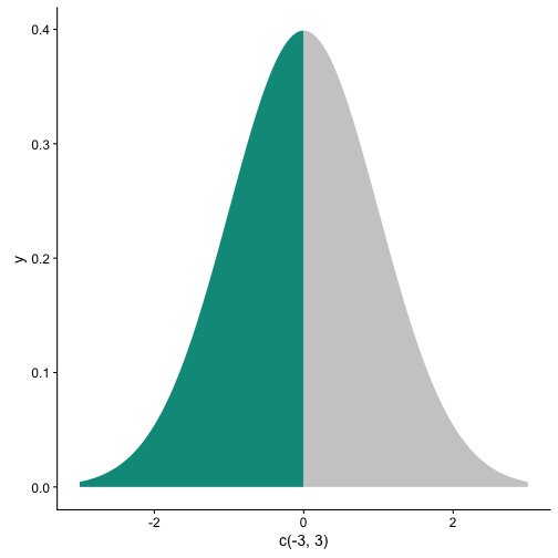
Shading values/areas under the normal curve is a quite frequent taks in eg educational contexts. Thanks to Hadley in this post, I found this easy solution.

library(ggplot2)

```r
ggplot(NULL, aes(c(-3,3))) +
  geom_area(stat = "function", fun = dnorm, fill = "#00998a", xlim = c(-3, 0)) +
  geom_area(stat = "function", fun = dnorm, fill = "grey80", xlim = c(0, 3))

plot of chunk unnamed-chunk-1

Simple, right?

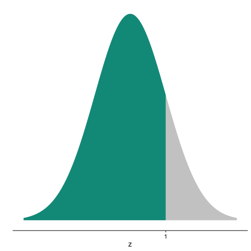
Some minor beautification:

 ggplot(NULL, aes(c(-3,3))) +
  geom_area(stat = "function", fun = dnorm, fill = "#00998a", xlim = c(-3, 1)) +
  geom_area(stat = "function", fun = dnorm, fill = "grey80", xlim = c(1, 3)) +
  labs(x = "z", y = "") +
  scale_y_continuous(breaks = NULL) +
  scale_x_continuous(breaks = 1)

plot of chunk unnamed-chunk-2

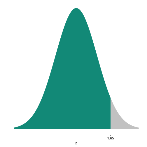
And some other quantiles:

ggplot(NULL, aes(c(-3,3))) +
  geom_area(stat = "function", fun = dnorm, fill = "#00998a", xlim = c(-3, 1.65)) +
  geom_area(stat = "function", fun = dnorm, fill = "grey80", xlim = c(1.65, 3)) +
  labs(x = "z", y = "") +
  scale_y_continuous(breaks = NULL) +
  scale_x_continuous(breaks = 1.65)

plot of chunk unnamed-chunk-3

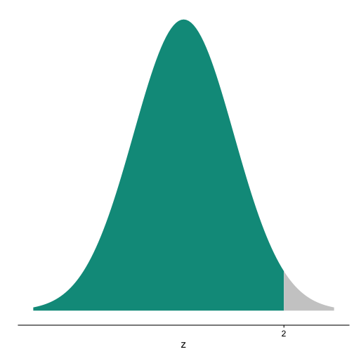
ggplot(NULL, aes(c(-3,3))) +
  geom_area(stat = "function", fun = dnorm, fill = "#00998a", xlim = c(-3, 2)) +
  geom_area(stat = "function", fun = dnorm, fill = "grey80", xlim = c(2, 3)) +
  labs(x = "z", y = "") +
  scale_y_continuous(breaks = NULL) +
  scale_x_continuous(breaks = 2)

plot of chunk unnamed-chunk-3

More on programming with dplyr: converting quosures to strings

In this post, we have programmed a simple function using dplyr’s programming capabilities based on tidyeval; for more intro to programming with dplyr, see here.

In this post, we’ll go one step further and programm a function where a quosure will be turned to a string. Why this? Because quite a number of functions out there except strings as input parameters.

Libraries

library(tidyverse)
library(stringr)

Data example

Say, we have a string where we search for a word stem. However this stem does not appear in its “stem” form, but always with some suffixes. Let our stem be “spd” (the name of the German Social-Democratic party), and (for simplicity), we’ll assume two “instances” of “spd” that occurr with suffix, ie., “spdbt” and “spdde”. (I was just working on a text mining on Tweets of German politiicians, hence the example).

data <- c("spdde", "sdf", "sdf", "fdds", "spdde", "dsf", "spdbt", "df") %>% as_tibble
stem <- "spd"

Task 01: Extract the “spd” stem out of the data

Non-programmatically, ie., interactively, this is quite straight-forward. Some knowledge of Regex is helpful to render the task a bit more general:

data %>% 
  mutate(is_instance = str_detect(string = value, pattern = "spd\\w+"),
         instance = str_match(value, "spd\\w+"))
## # A tibble: 8 x 3
##   value is_instance instance
##   <chr>       <lgl>    <chr>
## 1 spdde        TRUE    spdde
## 2   sdf       FALSE     <NA>
## 3   sdf       FALSE     <NA>
## 4  fdds       FALSE     <NA>
## 5 spdde        TRUE    spdde
## 6   dsf       FALSE     <NA>
## 7 spdbt        TRUE    spdbt
## 8    df       FALSE     <NA>

\\w means “find a word-character” (ie., letter or digit), and + means that at least 1 hit is expected. pattern is the pattern to be looked for and string defines the string where to search for the pattern.

Task 02: Make it a function

Obviously, a function is much more general. Say we have 10 parties we would like to warp through; it becomes tedious to repeat that code many times. We will want a function. How to do that with dplyr?

Let’s define a function with input parameters df for the name of the dataframe, col for the name of the column where the stemming is performend, and stem, the term to be stemmed.

stemm_col <- function(df, col, stem){
  
  col <- enquo(col)
  col_name <- quo_name(enquo(col))
  stem_name <- quo_name(enquo(stem))

  df %>% 
    mutate(stemmed = str_extract(string = !!col,
                                pattern = paste0(stem_name,"\\w+"))) -> output
  
  return(output)
}

See whether it runs:

stemm_col(df = data, col = value, stem = "spd")
## # A tibble: 8 x 2
##   value stemmed
##   <chr>   <chr>
## 1 spdde   spdde
## 2   sdf    <NA>
## 3   sdf    <NA>
## 4  fdds    <NA>
## 5 spdde   spdde
## 6   dsf    <NA>
## 7 spdbt   spdbt
## 8    df    <NA>

Bit by bit explanation

  • col <- enquo(col) – Take the parameter col, and just remember, R, that it is an expression, in this case, the parameter of a function, denoting a column.

  • col_name <- quo_name(enquo(col)) – Now turn col (an expression) to a string, because the function further down (str_extract) expects a string.

  • str_extract(string = !!col,... – Hey R, when you extract the strings, you need to know which string to search. OK, take col which is an expression, and now evaluate it (indicated by !!), in this case, understand that it’s a column. Now go get the values.

Main idea

When working with NSE, it is important to distinguish between expression, strings and evaluation. Using NSE, we can look at the parameters of a function, and grap the parameters before they are evaluated. That’s why the parameters need not be well-behaved, importantly, they do not need to have quotation marks, which saves typing for the user.

From the perspective of the R-interpreter (the machine), the steps of action looks more or less like this:

  1. Look at the parameters of the function

  2. Save the parameters not as strings, not as variables, but as expressions (via enquo)

  3. Convert the expression to a string (via quo_name) or, eventually,

  4. Evaluate it, ie., unquote (let the function to its job) via !! (called bang-bang) or via UQ.

In this post, we will explore some date and time parsing. As an example, we will work with weather data provided by City of Nuremberg, Environmental and Meteorological Data.

We will need these packages:

library(tidyverse)  # data reading and wrangling
library(lubridate)  # working with dates/times

First, let’s import some precipitation data:

file_name <- "~/Downloads/export-sun-nuremberg--flugfeld--airport--precipitation-data--1-hour--individuell.csv"
rain <- read_csv2(file_name,
                 skip = 13,
                 col_names = FALSE)
## Warning in rbind(names(probs), probs_f): number of columns of result is not
## a multiple of vector length (arg 1)
## Warning: 300 parsing failures.
## row # A tibble: 5 x 5 col     row   col expected actual expected   <int> <chr>    <chr>  <chr> actual 1  1643    X2 a double      - file 2  1644    X2 a double      - row 3  1645    X2 a double      - col 4  1646    X2 a double      - expected 5  1647    X2 a double      - actual # ... with 1 more variables: file <chr>
## ... ................. ... ............................. ........ ............................. ...... ............................. .... ............................. ... ............................. ... ............................. ........ ............................. ...... .......................................
## See problems(...) for more details.
colnames(rain) <- c("date_time", "precip")

As there was some strange, non-UTF8 character in line 12, we just skipped this line. As this was the row with the column names, we informed read_csv that there are no col_names (using col_names = FALSE). Also, some missing data occured. Luckily, readr takes care (despite of a lot of warning output).

Unfortunately, R has not yet reckognized that the first column consists of a date/time object. So let’s tell her:

rain$dt <- parse_date_time(rain$date_time, orders="dmy HM")

The parameter order tell R, that the format of date_time is day month year (hence dmy), followed by hour and minute (hence HM). Now let’s spread the date/time to several columns:

rain %>%
  select(-date_time) %>%
  mutate(day = day(dt),
         month = month(dt),
         year = year(dt),
         hour = hour(dt)) -> rain

Let’s give each day a number, first day in record is #1, second day #2, and so on.

rain$date <- date(rain$dt)

first_day <- min(rain$date)
last_day <- max(rain$date)

rain$day_ID <- rain$date - min(rain$date)

OK, now let’s look at the precipitation in Nuremberg.

How many dry days (no rain) have there been in 2016?

rain %>%
  group_by(day_ID) %>%
  summarise(precip_day_sum = sum(precip)) %>%
  filter(precip_day_sum == 0) %>%
  nrow -> n_dry_days

n_dry_days
## [1] 207

Oh, 207 out of 366 days no rain, ie., 0.55. BTW: It was a leap year, that’s why I put 366 days.

rain %>%
  group_by(day_ID) %>%
  slice(1) %>% nrow
## [1] 366

Easy enought, this little sweet function tells us whether a given year was a leap year or not.

leap_year(2016)
## [1] TRUE

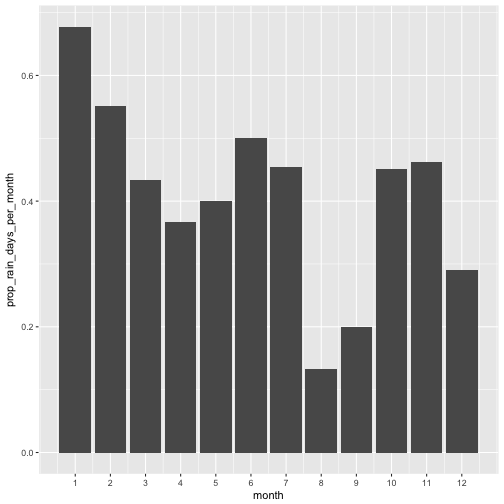
Let’s visualize whether a day was dry or not. First, we compute a variable rain_today.

rain %>%
  group_by(year, month, day, day_ID) %>%
  summarise(rain_today = any(precip != 0)) %>%
  filter(!is.na(rain_today)) %>%
  group_by(month) %>%   
  summarise(prop_rain_days_per_month = sum(rain_today)/n()) %>%
  ggplot() +
  aes(x = month, y = prop_rain_days_per_month) %>%
  geom_col() +
  scale_x_continuous(breaks = 1:12)

plot of chunk unnamed-chunk-9

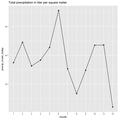
August and September then were quite dry, it appears. Let’s look at the amount of precipitation for comparison.

rain %>%
  group_by(month) %>%
  summarise(precip_mean_today = sum(precip, na.rm = T)) %>%
  ggplot(aes(x = month, y = precip_mean_today)) +
  geom_line() +
  geom_point() +
  scale_x_continuous(breaks = 1:12) +
  labs(title = "Total precipitation in liter per square meter")

plot of chunk unnamed-chunk-10

For the fun of it, let’s prepare a more nuanced picture.

rain %>%
  ggplot +
  aes(x = date, y = hour, fill = precip) +
  geom_tile() +
  scale_fill_distiller(palette = "Spectral") +
  scale_x_date(date_breaks = "1 month", date_labels = "%b")

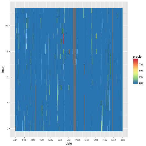
plot of chunk unnamed-chunk-11

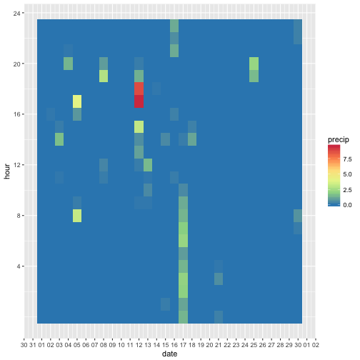
Hey, in June there must have been some heavy raining. Let’s zoom in.

rain %>%
  filter(month == 6) %>%
  ggplot +
  aes(x = date, y = hour, fill = precip) +
  geom_tile() +
  scale_fill_distiller(palette = "Spectral") +
  scale_x_date(date_breaks = "1 day", date_labels = "%d") +
  scale_y_continuous(breaks = c(4, 8, 12, 16, 20, 24))

plot of chunk unnamed-chunk-12

Most of the days in June were dry, but on one day, heave rains occurred on the 12th or 13th in the late afternoon.

rain %>%
  filter(precip > 7)
## # A tibble: 4 x 8
##   precip                  dt   day month  year  hour       date   day_ID
##    <dbl>              <dttm> <int> <dbl> <dbl> <int>     <date>   <time>
## 1    7.4 2016-05-29 21:00:00    29     5  2016    21 2016-05-29 149 days
## 2    9.5 2016-06-12 17:00:00    12     6  2016    17 2016-06-12 163 days
## 3    8.7 2016-06-12 18:00:00    12     6  2016    18 2016-06-12 163 days
## 4    7.2 2016-07-13 15:00:00    13     7  2016    15 2016-07-13 194 days

On June, 12th between 17:00 and 19:00 CEDT, a lot of rain came down in Nuremburg.

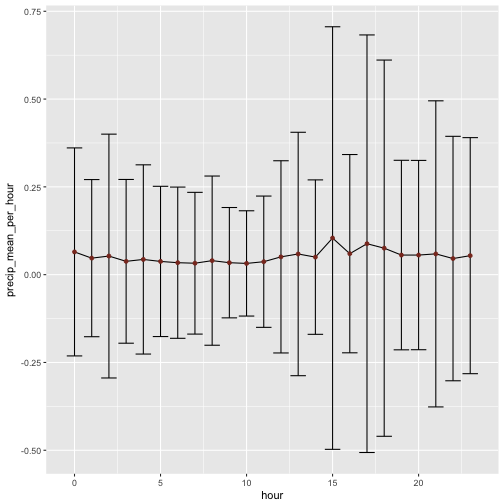
Is there a preference for time in terms of precipitation? Maybe it rather rains in the late afternoon in general?

rain %>%
  group_by(hour) %>%
  summarise(precip_mean_per_hour = mean(precip, na.rm = T),
            precip_sd_per_hour = sd(precip, na.rm = T)) %>%
  ggplot +
  aes(x = hour, y = precip_mean_per_hour) +
  geom_line() +
  geom_errorbar(aes(ymin = precip_mean_per_hour - precip_sd_per_hour,
                    ymax = precip_mean_per_hour + precip_sd_per_hour)) +
  geom_point(color = "tomato4")

plot of chunk unnamed-chunk-14

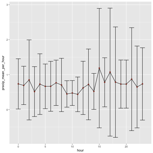
Hm, not much difference between the hours. But the variability seems to differ quite some bit. Would that picture change if we consider only days with precipation?

rain %>%
  filter(precip != 0) %>%
  group_by(hour) %>%
  summarise(precip_mean_per_hour = mean(precip, na.rm = T),
            precip_sd_per_hour = sd(precip, na.rm = T)) %>%
  ggplot +
  aes(x = hour, y = precip_mean_per_hour) +
  geom_line() +
  geom_errorbar(aes(ymin = precip_mean_per_hour - precip_sd_per_hour,
                    ymax = precip_mean_per_hour + precip_sd_per_hour)) +
  geom_point(color = "tomato4")

plot of chunk unnamed-chunk-15

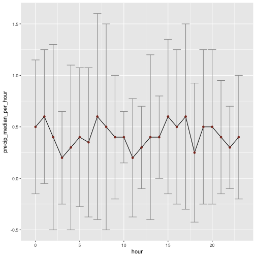
Not too much difference in the overall pattern. But what about if we look at the median and IQR, instead of mean and sd?

rain %>%
  filter(precip != 0) %>%
  group_by(hour) %>%
  summarise(precip_median_per_hour = median(precip, na.rm = T),
            precip_iqr_per_hour = IQR(precip, na.rm = T)) %>%
  ggplot +
  aes(x = hour, y = precip_median_per_hour) +
  geom_line() +
  geom_errorbar(aes(ymin = precip_median_per_hour - precip_iqr_per_hour,
                    ymax = precip_median_per_hour + precip_iqr_per_hour),
                color = "grey60") +
  geom_point(color = "tomato4")

plot of chunk unnamed-chunk-16

That the pattern breaks down essentially. Not that much difference between the hours left. Maybe 10:00 is rather dry, but that may be sampling errror of this year.

Recently, since dplyr <= 0.6.0 a new way of dealing with NSE was introduced, called tidyeval. As with every topic that begs our attention, the question “why bother” is in place. Theone answer is “you’ll need this stuff if you want to lock dplyr verbs inside a function”. Once you like dplyr and friends, a natural second step is to use the ideas not only for interactive use, but for more “programming” type, ie., writing functions.

The topic of this post is to explain some of the ‘tidyeval’ thinking. That is, let’s write a function using tidyeval thinking.

Build a function using tidyeval ideas

As an example, assume we want to have a function that takes two numeric vectors (ie., two groups), performs all pairwise comparisons (>), and returns the proportion ‘favorable’ for the first group. Say, out of 20 comparisons, 16 showed that group1 > group2. Hence, the ‘proportion of favorable comparisons’ would be 16/20 or .8. This measure can be seen as an effect size for the Mann Whitney U Test, Wilcoxon Test or even some type of rank biserial correlation. See the nice paper on the “Simple Difference Formula” of Kerby 2014 for details and background.

First, load tidyverse.

library(tidyverse)

Let’s take the mtcars dataset, I know it’s boring, but instructive, I hope.

So, here comes the function prop_fav:

prop_fav <- function(df, value, group, g1, g2){
  value <- enquo(value)
  group <- enquo(group)


  df %>%
   filter((!!group) == g1) %>%
   select(!!value) %>%
   pull -> values_g1

  df %>%
    filter((!!group) == g2) %>%
    select(!!value) %>%
    pull -> values_g2

  values_g1 <- na.omit(values_g1)
  values_g2 <- na.omit(values_g2)

  comp_grid <- expand.grid(values_g1, values_g2)

  fav_vec <- comp_grid[["Var1"]] > comp_grid[["Var2"]]

  fav_sum <- sum(fav_vec)

  fav_prop <- fav_sum / nrow(comp_grid)

  return(fav_prop)

}

tidyeval steps explained

What did we do? Let’s look at the steps in turn:

# don't run these lines, only run function 'fav_prop'

value <- enquo(value)
group <- enquo(group)

With enquo we take the parameter of a function as expression. That means, we do not evaluate it, we just take the expression, leave it on hold, and use it later on.

Then we extract the values of group 1 and group2 out of the data frame (assumed tidy). In tidy data frames, each variable has its own column. So we need to do some work to get the values extracted.

Don’ t run the following lines, simply run the function ‘fav_prop’.

# don't run these lines, only run function 'fav_prop'

df %>%
   filter((!!group) == g1) %>%
   select(!!value) %>%
   pull -> values_g1

  df %>%
    filter((!!group) == g2) %>%
    select(!!value) %>%
    pull -> values_g2

See the !!; they mean “hey R, remember the expression I stored recently? Now take it, and ‘unquote’ it, that is, just run it!”. The double exclamation mark is just syntactic sugar for that phrase.

pull, also recently added to dplyr, pulls out a vector (column) out of a data frame.

And in the last bit, we take the two vectors, span a Cartesian product and do a comparison of each element. More bluntly, take the first value of group 1 and compare it with value 1 of group 2. Decide which is greater. Go on comparing value 1 with the rest of values in group 2. And then go on with the rest of the values of group 1 in the same manner.

Then we simple compute the proportion where a member of group 1 had a greater value than a member of group 2. The proportion resulting is a measure of the effect size for the difference in distribution of the two groups.

# don't run these lines, only run function 'fav_prop'

 comp_grid <- expand.grid(values_g1, values_g2)

  fav_vec <- comp_grid[["Var1"]] > comp_grid[["Var2"]]

  fav_sum <- sum(fav_vec)

  fav_prop <- fav_sum / nrow(comp_grid)

Convenience sourcing

For convenience, this function can be sourced like this:

source("https://sebastiansauer.github.io/Rcode/prop_fav.R")

Example time

Now, some examples. Comparing cars with 4 and 6 cylinders, how many of the 4 cylinder group has more horse power? Or, more precisely, “Out of 100 comparisons of 4 and 6 cyl cars, what’s the proportion of 4 cyl cars having more hp (than the 6 cyl group)?”.

prop_fav(df = mtcars, value = hp, group = cyl, g1 = 4, g2 = 6)
## [1] 0.06493506

About 6%. Accordingly, in ~94% of the comparisons, a 6 cyl car had more horse power.

prop_fav(df = mtcars, value = hp, group = cyl, g1 = 6, g2 = 4)
## [1] 0.9350649

Let’s look at extraversion, coming from this dataset:

# devtools::install_github("sebastiansauer/prada")
data(extra, package = "prada")

Let’s compare women and men to see how is more extrovert.

prop_fav(df = extra, value = extra_mean, group = sex, g1 = "Frau", g2 = "Mann")
## [1] 0.4867873

Women are about as extroverted as men.

What about the number of Facebook friends?

prop_fav(extra, n_facebook_friends, sex, g1 = "Frau", g2 = "Mann")
## [1] NA

Men have slightly more Facebook friends (in this sample).

Concluding thoughts

Note that this measure can be applied for non-metric, ie., ordinal variables. It is quite straight forward, that makes it easy to comprehend.

Using tidyeval can give a headache at start, but it is worthwhile if you want to dig deeper, and write your own functions. However, there may be some similar alternatives such as wrapr::let, see here.

This was just a tiny little start. Hadley Wickham’s book ‘Advances R’ gives a much more thorough introduction.
The Mann-Whitney U-Test is a test with a wide applicability, wider than the t-Test. Why that? Because the U-Test is applicable for ordinal data, and it can be argued that confining the metric level of a psychological variable to ordinal niveau is a reasonable bet. Second, it is robust, more robust than the t-test, because it only considers ranks, not raw values. In addition, some say that the efficiency of the U-Test is very close to the t-Test (.95). In sum: use the U-Test.

Idea of the U-Test

How is the test computed? In essence, that’s easy:

  1. Count the number of pairwise comparisons in your sample. Say you have two groups, with n1=5 and n2=4. Thus there are 20 comparisons in total.
  2. Now count the frequency group 1 “wins” a comparison (count 0.5 for ties). The resulting statistic can be called U.

How to achieve that in R? Try this code. Say we have two groups of runners (100m), and we record their running time (in seconds):

g1 <- c(9.9, 10.3, 11.5, 12.1, 23.3)
g2 <- c(13.2, 14.5, 15.2, 16.6)

Now let’s see all possible comparisons:

comp <- expand.grid(g1, g2)
names(comp) <- c("g1", "g2")
head(comp)
##     g1   g2
## 1  9.9 13.2
## 2 10.3 13.2
## 3 11.5 13.2
## 4 12.1 13.2
## 5 23.3 13.2
## 6  9.9 14.5

How man comparisons do we have?

nrow(comp)
## [1] 20

And now count how often members of g1 outperform members of g2, ie., we count the proportion of \(g1_i > g2_j\) for all \(i,j\).

I need the pipe for that…

library(tidyverse)
comp %>% 
  mutate(g1fasterg2 = g1 < g2) %>% 
  summarise(sum_g1fasterg2 = sum(g1fasterg2))
##   sum_g1fasterg2
## 1             16

So we now have the sum of “wins”; getting the proportion is easy, just divide by the number of comparisons.

Computing U the standard way

Let’s compare that to the more “traditional” way of computing U.

U is given by

\[U1 =\sum{g1} - \sum{min1}\]

where \(U1\) means the U statistic for g1, and \(min1\) is the minimal possible rank sum in g1. What’s the smallest possible rank sum if there are 2 observations in a group? 3. Because 1+2=3. If there are 5 runners in a group? 15. Because 1+2+3+4+5=15. So, in our case for g1, 15 is the minimal possible rank sum in g1. Now we now that if we get a rank sum of 15 that’s as possible as it can be.

Let’s compute the rank sums for each group.

First, build a dataframe:

df <- data.frame(
  runtime = c(g1, g2),
  groups = c(rep("g1", 5), rep("g2",4))
  )

Now transform the run time to ranks.

df %>% 
  mutate(ranks = min_rank(runtime)) -> df

Note that we are not considering ties here for the sake of simplicity.

Now compute the sum of ranks grouped by groups.

df %>% 
  group_by(groups) %>% 
  summarise(ranks_sum = sum(ranks))
## # A tibble: 2 x 2
##   groups ranks_sum
##   <fctr>     <int>
## 1     g1        19
## 2     g2        26

Applying the formula above we see that the rank sum for g1 is 19, subtracting the min rank of 15, we get a value of 4. This number is equivalent to saying that out of 20 comparisons, g1 lost 4 (and won 16). U is obviously synonymous to saying “how many comparisons were lost”.

For g2, similarly: 26 - 10 = 16, so 16 (out of 20) comparisons were lost.

Now, the proportion of won (or lost) comparisons is of course more telling than the absolute value, seen from a practical point of view. This amounts to saying that the proportion of won/lost comparisons is some kind of effect size. See details for this idea in the paper of Kerby (Kerby, D. S. (2014). The Simple Difference Formula: An Approach to Teaching Nonparametric Correlation. Comprehensive Psychology, 3, 11.IT.3.1. http://doi.org/10.2466/11.IT.3.1), and the 1992 paper of McGraw and Wong (McGraw, K. O., & Wong, S. P. (1992). A common language effect size statistic. Psychological Bulletin, 111(2), 361–365. http://doi.org/10.1037/0033-2909.111.2.361). That’s were the ideas presented here stem from (as far as I am involved).

The proportion of favorable comparisons can be gauged a “common language effect size” (CLES).

In our example, the effect size (CLES) would amount to 16/20 = 80% (.8). For the sake of a memorable example, let’s say that g1 are “doped runners” and g2 are “normal runners”.

It’s quite straight forward to say “doped runners outperform normal runners in 80 of 100 cases”.

As an effect size for non-parametric two-group comparison scenarios are quite often neglected in standard text books, I think it is helpful to ponder the CLES idea presented by Kerby, and put forward earlier by McGraw and Wong.