
This blog has moved to https://data-se.netlify.com/
Adios, Jekyll. Hello, Blogdown!
This blog has moved to https://data-se.netlify.com/
Adios, Jekyll. Hello, Blogdown!
Sie arbeiten bei der Flughafenaufsicht von NYC. Cooler Job.
library(nycflights13)
data(flights)
library(mosaic)
Die Aufsichtsbehörde zieht eine Probe von 100 Flügen und ermittelt die “typische” Verspätung.
set.seed(42)
sample(flights$arr_delay, size = 100) -> flights_sample
Und berechnen wir die typischen Kennwerte:
favstats(~flights_sample, na.rm = TRUE)
#>  min     Q1 median    Q3 max      mean      sd  n missing
#>  -51 -18.75     -5 11.75 150 0.4387755 31.1604 98       2
Ob $n=3$ ausreichen würde? Wäre billiger. “Fühlt” sich klein an…
set.seed(42)
sample(flights$arr_delay, size = 3) -> flights_small
favstats(~flights_small, na.rm = TRUE)
#>  min  Q1 median   Q3 max      mean       sd n missing
#>  -34 -28    -22 -0.5  21 -11.66667 28.91943 3       0
Hm, deutlich ungenauer.
Die Flughafenbetreiber beschweren sich. Die Stichprobe sei “nicht repräsentativ”; es sei “dumm gelaufen”.
Wie repräsentativ ist die Stichprobe? Keine Ahnung. Dazu müssten wir die Grundgesamtheit kennen. Die kennt man normalerweiß nicht.
In diesem Fall ausnahmsweise schon:
favstats(~arr_delay, data = flights, na.rm = TRUE)
#>  min  Q1 median Q3  max     mean       sd      n missing
#>  -86 -17     -5 14 1272 6.895377 44.63329 327346    9430
Median und MW der Sichprobe treffen die Wirklichkeit (Grundgesamtheit) “ganz gut”. Max und Min kaum.
Die Stichprobe entspricht der “typischen” Verspätung ganz gut. Ohne großes Aufsehen einigt man sich im Hinterzimmer. Kuh vom Eis.
Die Presse bekommt eine weitere Stichprobe zugespielt: Mittlere Verspätung in NYC sei 42 Minuten ($n=100$)! Der Bürgermeister tobt. So lahm? Schlimmer als die Deutsche Bahn. Sie müssen schnell was tun. Nur was…
Ob die Stichprobe überhaupt echt ist?
Sie ziehen viele vergleichbare Stichprobe aus der Grundgesamtheit (flights) und schauen, wie oft so ein Wert wie 42 als Mittelwert vorkommt!
Sagen wir, wir ziehen 10000 Stichproben und rechnen jeweils die mittlere Verspätung aus.
In wie vielen Stichproben ist die Verspätung 42 Minuten oder noch größer???
do(10000) * mean(sample(flights$arr_delay,
                        size = 100),
                 na.rm = TRUE) -> flights_vtlg
Schauen wir, wie oft 42 vorkommt:
gf_histogram(~mean, data = flights_vtlg)

Praktisch nie! Fast keine Stichprobe hatte eine mittlere Verspätung von 42 Minuten.
Wir könenn mit hoher Sicherheit ausschließen, dass die Stichprobe echt ist! Der Bürgermeister überlegt öffentlich, Ihnen einen Orden zu verpassen (aber keine Gehaltserhöhung).
Das Histogramm oben zeigt die Verteilung der 10000 Stichproben, die wir gerade gezogen haben (Danke, R). Man nennt es eine Stichprobenverteilung.
Die genauen Kennwerte dieser Stichprobenverteilung lauten:
favstats(~mean, data = flights_vtlg, na.rm = TRUE)
#>       min       Q1   median       Q3      max     mean       sd     n
#>  -7.43299 3.677004 6.567716 9.721649 33.42105 6.850973 4.528796 10000
#>  missing
#>        0
Jetzt können wir genau sagen, wie die typische Stichprobe an New Yorker Verspätungne aussieht: Mittlere Verspätung: Etwa 7 Minuten (arith. Mittel); sd beträgt etwa 5 Minuten.
Sagen wir, die 2.5% Stichproben mit der geringsten und die 2.5% Stichproben mit der höchsten Verspätung sind “ungewöhnlich”:
quantile(~mean, data= flights_vtlg,
         probs = c(.025, .975))
#>      2.5%     97.5%
#> -1.234694 16.394142
Ah: Stichproben mit weniger als -1.24 Minuten und Stichproben mit mehr als 16 Minuten sind “ungewöhnlich”. Alles dazwischen ist “normal”.
Nettes Beispiel. Aber in Wirklichkeit haben wir praktisch nie die Grundgesamtheit, nur unsere einsame, einzige Stichprobe. Beispiele:
Die Grundgesamtheit ist in der Praxis oft unbekannt.
Der Trick lautet: Wir tun so, als sei unsere einzige Stichprobe die Grundgesamtheit. Dann machen wir weiter wie gerade: Wir ziehen viele Stichproben aus ihr.
Diese Idee nennt man Bootstrapping. Probieren wir es aus. Wichtig ist, immer mit Zurücklegen zu ziehen. Stellen Sie sich vor, jedes Element der Stichprobe kommt unendlich oft darin vor. Das ist ja die Idee einer Grundgesamtheit. Ziehen mit Zurücklegen ist die Umsetzung dieser Idee.
Mit resample geht das:
resample(flights_small)
#> [1] 21 21 21
resample(flights_sample)
#>   [1] -26  -5 -41 -27   9 -16  13  27  -4  -8   3   7   4  20  -5 -19  21
#>  [18] -20  25  -1   9  -1 -18 -20 -13 -21  -8  37   0  37 -13  -6  -8 -20
#>  [35]  -9 -28  -6 -39  -6  43 -19  32 -28 -29  -1  19  50  -3 -28 -28 -12
#>  [52]  -3  -5   3   8 -19 -41  32  27 -19  12 -16 -41 -13  -5 -22 -11  -9
#>  [69]  27  -9  NA -21  25  20  -6 -34  25 -13  27  -6 -22  -5 -20  27 -34
#>  [86]  -5  -5  -1 -31 -26   5   0   7 -15  16 -16 -14  -1 -13  23
Was ist der Mittelwert?
mean(resample(flights_sample), na.rm = TRUE)
#> [1] -0.4343434
Kann man übrigens auch so schreiben:
resample(flights_sample) %>% mean(na.rm = TRUE)
#> [1] 0.43
Wir wiederholen diesen Schritt oft, sagen wir 10000 Mal:
flights_boot <- do(10000) * mean(resample(flights_sample), na.rm = TRUE)
Und schauen uns das Histogramm an:
#rename(flights_boot, arr_delay_avg = "mean") -> flights_boot
gf_histogram(~mean, data = flights_boot)

Die genauen Statistiken sehen so aus:
favstats(~mean, data = flights_boot, na.rm = TRUE)
#>        min        Q1    median      Q3      max     mean       sd     n
#>  -10.36082 -1.693878 0.3787755 2.56701 12.81818 0.477432 3.127597 10000
#>  missing
#>        0
Hey, wie durch Zauberei haben wir mit unserer Bootstrap-Methode eine Verteilung erhalten, die der Stichprobenverteilung sehr ähnlich ist. Anhand der Bootstrap-Verteilung können wir jetzt sagen, was eine “typische” Stichprobe ist und ob die 42-Minuten-Stichprobe zu den ungewöhnlichen Stichproben gehört.
quantile(~mean, data= flights_boot, probs = c(.025, .975))
#>      2.5%     97.5%
#> -5.316582  6.909258
Stichproben mit mehr als 22 Minuten Verspätung gehören zu den “ungewöhnlihen” Stichproben; die 42-Minuten-Stichprobe ist also ungewöhnlich.
Wenn jemand sagt, heute (am 17. November) hätte es in Novisibirsk 27 Grad, dann wäre das “ungewöhnlich” für Novisibirsk und diese Jahreszeit. Oder: die Daten stammen nicht aus Novisibirsk (das ist freundlicher als zu sagen, sie seien gefälscht).
So die Pressemitteilung, die der Bürgermeister schließlich herausgibt. Er lässt sich so zitieren: “42 Minuten Verspätung sind seehr ungewöhnlich für NYC. Daher sind diese Daten vermutlich gef… äh stammen nicht von unseren Flughäfen”.
Mit der Bootverteilung kann man einschätzen, wie “typisch” eine Stichprobe für eine Grundgesamtheit ist. Außerdem kann man sagen, ob eine Stichprobe “ungewöhnlich” für eine Grundgesamtheit ist.
The tidyeval framework is a rather new, and in parts complementary, framework to dealing with non-standarde evaluation (NSE) in R. In short, NSE is about capturing some R-code, witholding execution, maybe editing the code, and finally execuing it later and/or somewhere else.
This post borrows heavily by Edwin Thon’s great post, and this post by the same author.
In addtion, most of the knowledge is derived from Hadley Wickham’s book Advanced R.
The typical base R culprits are eval(), and quote() or substitute(),
respectively.
library(tidyverse)  # load tidyeval too
library(rlang)  # more on tidyeval
library(pryr)  # working with environments
##
## Attaching package: 'pryr'
## The following object is masked from 'package:rlang':
##
##     bytes
## The following objects are masked from 'package:purrr':
##
##     compose, partial
And why should I bother?
Let’s look at some border case that show the difference quite strikingly.
Consider this base nse code:
base_NSE_fun <- function(some_arg) {
  some_var <- 10
  quote(some_var + some_arg)
}
base_NSE_fun(4) %>% eval()
## Error in eval(.): object 'some_var' not found
It does not work. eval() has no idea about the environment in which some_var is defined. (And in addition, quote() will take its arguments too literally, but we spare that for later.)
We might had expected the code above to work, however. That’s where tidyeval comes into play:
See here:
tidy_eval_fun <- function(some_arg) {
  some_var <- 10
  quo(some_var + some_arg)
}
tidy_eval_fun(4) %>% rlang::eval_tidy()
## [1] 14
Does work. With tidyeval, the environment of the variables are memorized. With base R, the environment is forgotton.
What’s the enclosing environment of eval()? We can get hold of that environment using the function environment():
environment(eval)
## <environment: namespace:base>
What’s that for a strange environment? Well, that’s the NAMESPACE of package base, the exported objects of that package. A namespace is useful so the searchpath will not be cluttered by too many objects. Using a namespace we can define which objects should be made (easily) accessible to the users.
But in this environment, for sure, we will not have put some variable. How comes that this code does wor:
vanilla_x <- 1
eval(vanilla_x)
## [1] 1
What’s the environment of vanilla_x? We can access the enclosing environment of some object using this code:
pryr::where("vanilla_x")
## <environment: R_GlobalEnv>
So, if eval() looks in the namespace of base how comes that it finds some object in the global environment?
The answer is called lexical scoping. There’s a chain or ladder of enclosing environments, where the value is looked for. The total of this chaining is the search path.
Hadley Wickham illustrates this chain using this diagram in this chapter of Adv R:
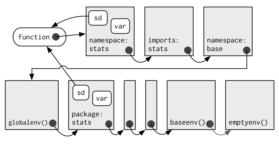
Each arrow coming from a grey dot refers to the enclosing environment of some object or function. The enclosing environment is the “home” environment, where the object was created.
We see that each object has an environment, and each environment has exactly one “parent” environment - with the notably execption of the emptyenv which is the first “ancestor” of this sequence.
A function can and does have four environments:
substitute() can and cannot dosubstitute() is the counterpart of quote() for use within functions. Do not use quote() within functions, use substitue() instead (or the tidyeval counterpart).
Consider:
base_eval_fun2 <- function(some_arg) {
  some_var <- 10
  substitute(some_var + some_arg)
}
base_eval_fun2(4) %>% rlang::eval_tidy()
## [1] 14
Great! Appears to work, does is not? Not exactly. Look what the function
call tidy_eval_fun2(4) is actually returning:
base_eval_fun2(4)
## 10 + 4
The result is quite hard coded (Thanks Edwin for pointing that out!). Compare the tidyeval variant:
tidy_eval_fun2 <- function(some_arg) {
  some_var <- 10
  quo(some_var + some_arg)
}
tidy_eval_fun2(4)
## <quosure: local>
## ~some_var + some_arg
Now we do not get the “hard” values but the variables AND their environment is carried over. We might change the expression or carry it to another environment where some_arg has some other value.
It would be useful to have a RMarkdown template for typical (academic) reports such as class assigments and bachelor/master thesises. The LaTeX class “report” provides a suitable format for that. This package provides a simple wrapper around this class built on the standard pandoc template.
Yart, ie, this package leans on earlier work by Aaron Wolen in his pandoc-letter repository, and extends it for use from R via the rmarkdown package. The structure of this package is heavily inspired by Dirk Eddenbuettel’s nice tamplate package linl.
The bulk of the work has been done by John McFarlane’s pandoc, Donald Knuth’s LaTeX, and Yihui Xie’s knitr, along with the earlier work of many.
Yart is a R package that provides a RMarkdown template suitable for (academic) reports. Users write basically only content with a few metadata (such as title, school’s name etc), and the template translates all that to LaTeX which is then being rendered to a PDF file.
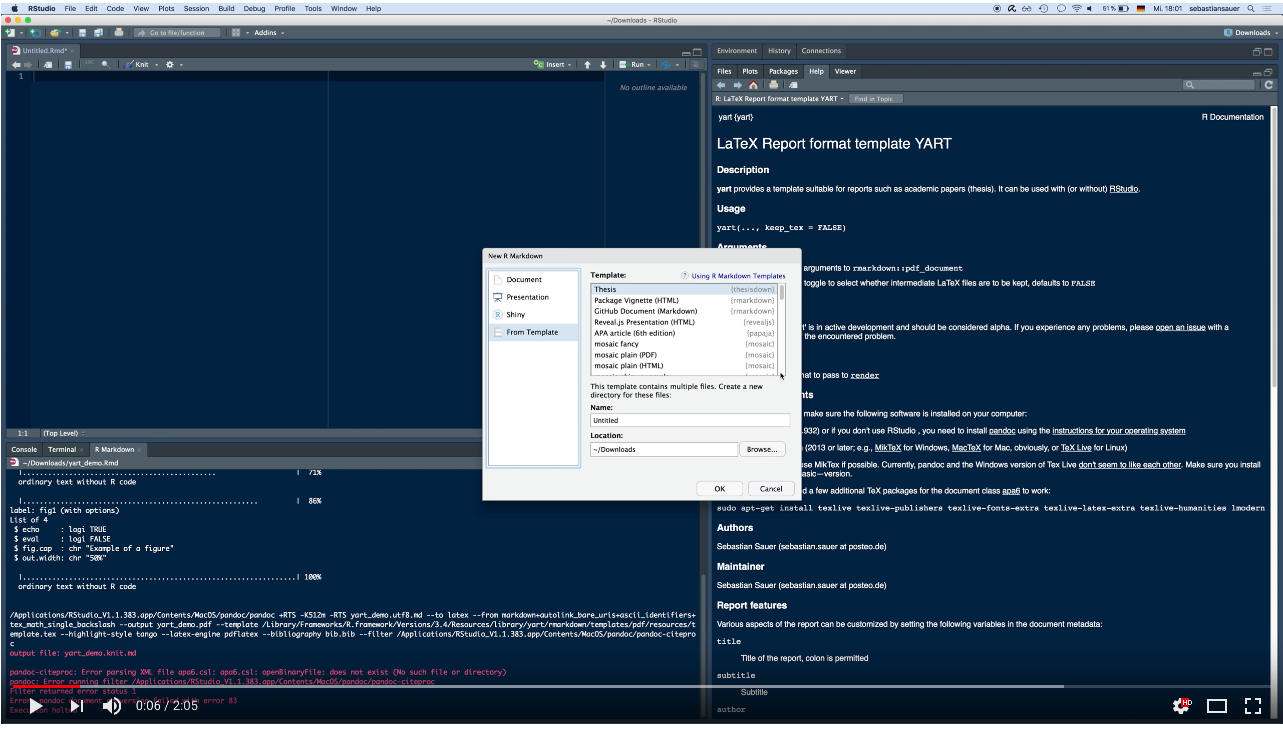
The following screenshot shows on the left hand side the raw markdown file and on the right hand side the compiled pdf paper.
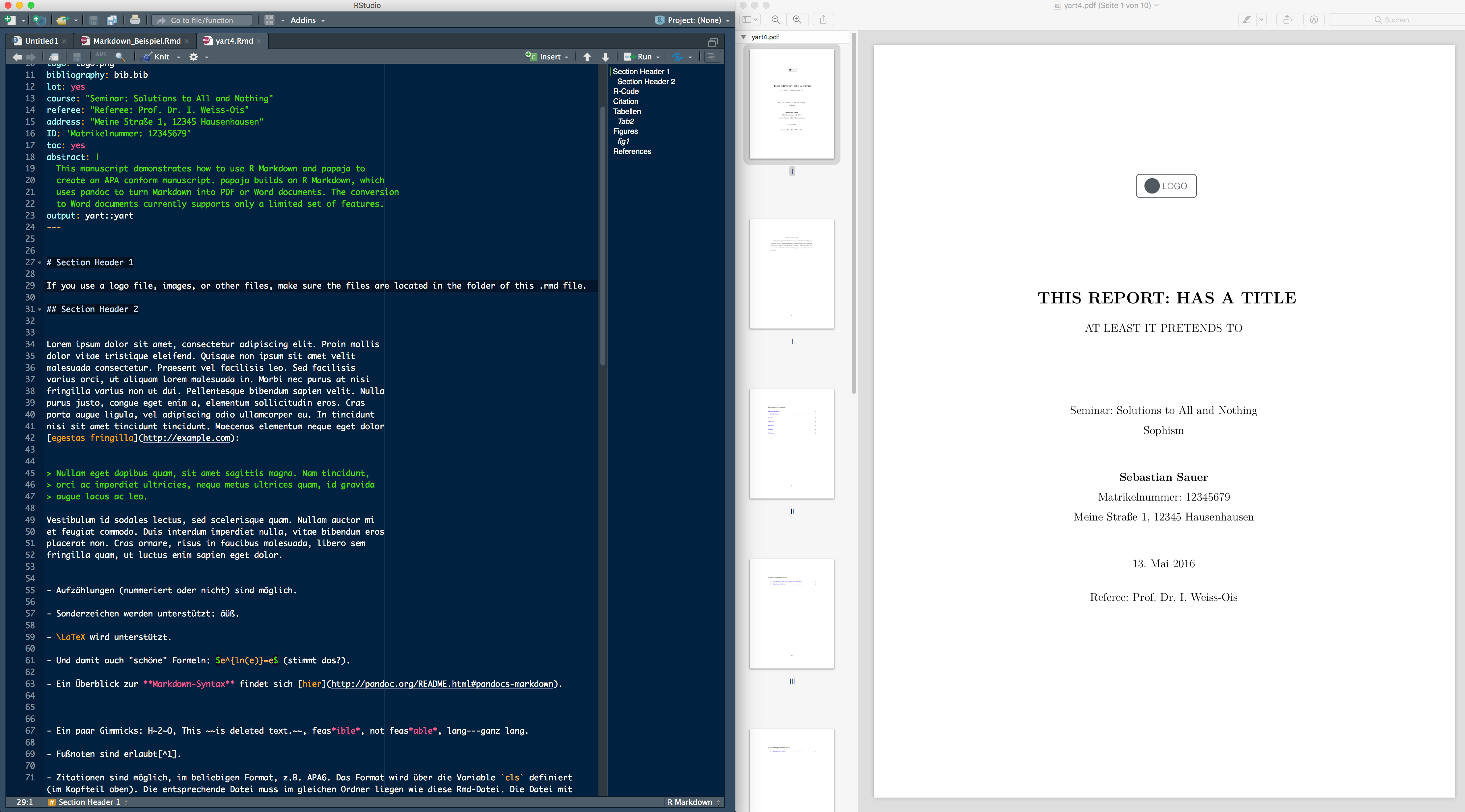
Being built on Pandoc, yart provides the typical features of Pandoc’s Markdown, inculding citation, figures, tables and references thereto – and basically, via a template, the fully featured LaTeX beauty. Being built on RMarkdown/knitr, R can be knitted into the text document.
The specific add-on of this template is that it configurates a LaTeX template suitable for (academic) reports so that the user does not have to deal with the LaTeX peculiarities and can focus on writing/contents. There are a number of levers which can be adapted by the used in the yart template including author name, title, subtitle, address, date, referee’s name, assignment name, school’s name, due date.
Install via R from Github:
devtools::install_github("sebastiansauer/yart")
LaTeX needs to be installed.
The skeleton creates a very simple letter.
Several formatting defaults are in use. See help(yart) for a
complete list and default values.
The vignette example is a little more featureful and shows how to include a letterhead on-demand, a signature, and a few formatting settings.
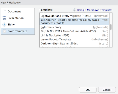
First, open as a Markdown template via RStudio via File > New File > RMarkdown > From Template > YART. The template list or Rmarkdown should feature the YART template upon the package installation:
Second, “knit” to document to pdf:
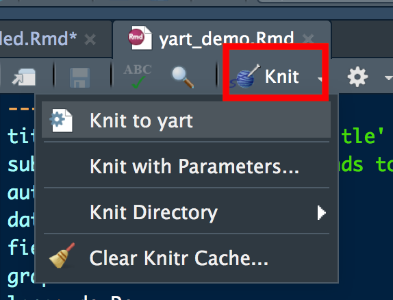
or use code such as
library(rmarkdown)
draft("my_report.Rmd", template="pdf", package="yart", edit=FALSE)
render("my_report.Rmd")
to create a first draft of a new my_report.Rmd.
Please report issues here along with a reproducible example if possible.
A number of R packages for RMarkdown templates for PDF documents are available including
Sebastian Sauer
GPL-3 for this package, the work in pandoc-letter, as well as underlying Pandoc template.
Recently, I’ve put a package on Github featureing some social science data set. Some data came from official sites; my contribution was to clear ‘em up, and render comfortably accessable for automatic inquiry (nice header lines, no special enconding, flat csvs….). In other cases it’s unpublished data collected by friends, students of mine or myself.
Let’s check its contents using a function by Maiasaura from this SO post.
library(pradadata)
lsp <- function (package, all.names = FALSE, pattern) {
    package <- deparse(substitute(package))
    ls(pos = paste("package", package, sep = ":"), all.names = all.names,
        pattern = pattern)
}
So, as of today, this dataset are included:
data_in_pradadata <- lsp(pradadata)
data_in_pradadata
#>  [1] "cult_values"    "dating"         "elec_results"   "extra"
#>  [5] "extra_names"    "parties_de"     "socec"          "socec_dict"
#>  [9] "stats_test"     "wahlkreise_shp" "wellbeing"      "Werte"
#> [13] "wo_men"
Let’s check the help documentation for each object; the R code is inspired by Joshua Ulrich, see this SO post.
library(purrr)

data_in_pradadata %>%
  map(help) %>%
 # simplify %>%
  map(~tools:::Rd2txt(utils:::.getHelpFile(as.character(.))))
#> _S_c_h_w_a_r_t_z _C_u_l_t_u_r_a_l _V_a_l_u_e _O_r_i_e_n_t_a_t_i_o_n _S_c_o_r_e_s _f_o_r _8_0 _c_o_u_n_t_r_i_e_s
#>
#> _D_e_s_c_r_i_p_t_i_o_n:
#>
#>      Data based on Schwartz' theory of cultural values.
#>
#> _U_s_a_g_e:
#>
#>      cult_values
#>
#> _F_o_r_m_a_t:
#>
#>      a data frame with 83 rows and 10 variables:
#>
#>      country short country name, short form
#>
#>      country_long country name, long form
#>
#>      harmony Unity With Nature World at Peace
#>
#>      embedded Social Order, Obedience Respect for Tradition
#>
#>      hierarchy Authority Humble
#>
#>      mastery Ambition Daring
#>
#>      aff_auton affective autonomy; Pleasure
#>
#>      intel_auton intellectual autonomy; Broadmindedness Curiosity
#>
#>      egalitar egalitarianism; Social Justice Equality
#>
#> _D_e_t_a_i_l_s:
#>
#>      The following description is taken from <URL:
#>      http://latest-schwartz.wikidot.com/> (CC-BY-SA 3.0)
#>
#>      Data were collected between 1988 and 2000
#>
#>      There are 7 cultural dimensions in Schwartz
#>      theory:harmony,embeddedness,hierarchy,mastery,affective
#>      autonomy,intellectual autonomy,egalitarianism.
#>
#>      Embeddedness VS Autonomy:Embeddedness appears in situations where
#>      individuals are embedded in a collectivity and find meaning
#>      through social relationships,through identifying with the
#>      group,participating in its shared way of life,and striving toward
#>      its shared goals.In embeddedness societies personal interests are
#>      not seen as different from those of the group and high value is
#>      placed on preserving the status quo and avoiding individual
#>      actions or attitudes that might undermine the traditional order of
#>      things.Important values in such societies are social order,respect
#>      for tradition,security,obedience and wisedom.While autonomy refers
#>      to the situation where individuals are viewed as
#>      autonomous.bounded entities that are expected to cultivate and
#>      express their own preferences,feelings,ideas,and abilities and
#>      find meaning in their own uniqueness.Autonomy is further broken
#>      down into two categories:intellectual autonomy which refers to the
#>      independent prusuit of ideas ,intellectual derections and
#>      rights;affective autonomy,which refers to the independent pursuit
#>      of affectively positive experiences such as varied life,pleasure
#>      and enjoyment of life.
#>
#>      Hierarchy VS Egalitarianism:In hierarchical societies individuals
#>      and the resources associated with society are organized
#>      hierarchically and individuals within those societies are
#>      socialized to comply with the roles assigned to them in the
#>      hierarchy and subjected to sanctions if they fail to
#>      comply.Modesty and self-control are values associated with
#>      hierarchy.In egalitarian societies individuals are seen as moral
#>      equals and everyone shares the same basic interests as human
#>      beings.In egalitarian societies people are socialized to
#>      internalize a commitment to cooperate and to feel concern for
#>      everyone's welfare.Valued associated with egalitarian societies
#>      include socail justice and caring for the weaker members of the
#>      society,honesty,equality,sympathy and working for the good of
#>      others,social responsibility and voluntary cooperation in the
#>      pursuit of well-being or prosperity for others within the society.
#>
#>      Mastery VS Harmony:Mastery refers to the situation wher
#>      individuals value succeeding and getting ahead through
#>      self-assertion and proactively seek to master,direct and change
#>      the natural and social world to advance their personal interests
#>      and the interests of the groups to which they belong.Specific
#>      values associated with mastery include independence,fearlessness
#>      and daring,ambition and hard work,drive for success and
#>      competence.Harmony refers to the situation wher individuals are
#>      content to accept and fit into the natural and social world as
#>      they find it and seek to understand,preserve and protect it rather
#>      than change,direct or exploit it.Important values in societies
#>      where harmony is valued include world at peace,unity with
#>      nature,and protecting the environment.
#>
#>      Here are the conclusions of Schwartz theory:cultural value
#>      orientations can be inferred form mean values of individuals in
#>      societies;world composed of cultural regions,linked by
#>      history,geography,economics,religion;knowing how cultures differ
#>      gives tools for specific analysis of issuses in international
#>      contact;cultural value orientations relate in reciprocal causaltiy
#>      with key social structural,political,demographic features of
#>      society.
#>
#>      All items were collected on a -1 to +7 response scale.
#>
#>      Note: Three lines have added (for countries: can, ger, swi), with
#>      their values computed as (unweighted) average of the country
#>      parts.
#>
#> _S_o_u_r_c_e:
#>
#>      wikidot
#>
#> _R_e_f_e_r_e_n_c_e_s:
#>
#>      Schwartz, S. H. (2006). A theory of cultural value orientations:
#>      Explication and applications. Comparative sociology, 5(2),
#>      137-182.
#>
#> _R_e_s_u_l_t_s _f_r_o_m _a_n _e_x_p_e_r_i_m_e_n_t _o_n _s_t_a_t_u_s _s_y_m_b_o_l_s _a_n _d_a_t_i_n_g _s_u_c_c_e_s_s
#>
#> _D_e_s_c_r_i_p_t_i_o_n:
#>
#>      Data from an online dating/mating app experiment with IV "car as
#>      status symbol" (yes vs. no) and DV1 "matching" (number) and DV2
#>      "message sent" (number). The principal research question was
#>      whether a luxury sports car (BMW Z4) on the individual profile
#>      portrait photo at an online dating app would have an influence on
#>      the number of contact requests and messages sent to this profile.
#>      Care was taken that the profiles showed no difference besides the
#>      car.
#>
#> _U_s_a_g_e:
#>
#>      dating
#>
#> _F_o_r_m_a_t:
#>
#>      A data frame containing 5063 rows and 7 columns
#>
#>      strawperson Chr. DThere were 6 straw persons. ie., persons with a
#>           profile on the dating portal
#>
#>      sex Chr. Sex of strawperson
#>
#>      car Int. Whether a luxury sports car was on the profile picture or
#>           not
#>
#>      date Chr. Date mm/dd/yyyy
#>
#>      Age Int. Age
#>
#>      ID_hash Chr. Username anonymized
#>
#>      comm_type Type of communication by individuals: either matching or
#>           contact message
#>
#>      whr Numeric. Waist hip ratio of strawperson
#>
#>      beauty Subjective beauty rating of strawperson by rating committee
#>
#> _D_e_t_a_i_l_s:
#>
#>      This dataset was published here: <URL: https://osf.io/4hkjm/>.
#>
#> _S_o_u_r_c_e:
#>
#>      Please cite this dataset as: 'Sauer, S., & Wolff, A. (2016, August
#>      16). The effect of status symbols on success in online dating: an
#>      experimental study. Retrieved from osf.io/4hkjm'
#>
#> _D_a_t_a_f_r_a_m_e _c_o_n_t_a_i_n_i_n_g _t_h_e _r_e_s_u_l_t_s _o_f _t_h_e _2_0_1_7 _f_e_d_e_r_a_l _e_l_e_c_t_i_o_n_s
#> (_B_u_n_d_e_s_t_a_g_s_w_a_h_l)
#>
#> _D_e_s_c_r_i_p_t_i_o_n:
#>
#>      This dataset is published by the Bundeswahlleiter 2017 (c) Der
#>      Bundeswahlleiter, Wiesbaden 2017
#>      https://www.bundeswahlleiter.de/info/impressum.html
#>
#> _U_s_a_g_e:
#>
#>      elec_results
#>
#> _F_o_r_m_a_t:
#>
#>      A data frame containing 332 rows and 191 columns
#>
#>      district_nr Integer. Number of the electoral district
#>
#>      district_name Chr. Name of the electoral disctrict
#>
#>      parent_district_nr Int. Number of the parent district
#>
#>      registered_voters_1 Number of registered voters first vote
#>           \(Erststimme\), present election - 1
#>
#>      registered_voters_1 Number of registered voters first vote
#>           \(Erststimme\), previous election - 2
#>
#>      registered_voters_1 Number of registered voters second vote
#>           \(Zweitstimme\), present election - 3
#>
#>      registered_voters_1 Number of registered voters second vote
#>           \(Zweitstimme\), previous election - 4
#>
#>      votes_1 Number of eligible votes - 1
#>
#>      votes_2 Number of eligible votes - 2
#>
#>      votes_3 Number of eligible votes - 3
#>
#>      votes_4 Number of eligible votes - 4
#>
#>      votes_invalid_1 Number of invalid votes - 1
#>
#>      votes_invalid_2 Number of invalid votes - 2
#>
#>      votes_invalid_3 Number of invalid votes - 3
#>
#>      votes_invalid_4 Number of invalid votes - 4
#>
#>      votes_valid_1 Number of valid votes - 1
#>
#>      votes_valid_2 Number of valid votes - 2
#>
#>      votes_valid_3 Number of valid votes - 3
#>
#>      votes_valid_4 Number of valid votes - 4
#>
#>      CDU_1 Number of votes for CDU - 1
#>
#>      CDU_2 Number of votes for CDU - 2
#>
#>      CDU_3 Number of votes for CDU - 3
#>
#>      CDU_4 Number of votes for CDU - 4
#>
#> _D_e_t_a_i_l_s:
#>
#>      Data is made available for unrestricted use provided the source is
#>      credited.
#>
#>      Data presented here has been altered in the sense that it has been
#>      rendered more machine-friendly (one header row only, no special
#>      characters, no blanks in header line, etc.). Beside that, the data
#>      itself has not been changed in any way.
#>
#>      The columns are structures as follows. For each column AFTER
#>      'parent_district_nr', ie., from column 4 onward, 4 columns build
#>      one bundle. In each bundle, column 1 refers to the Erststimme in
#>      the present election; column 2 to the Erststimme in the previous
#>      election. Column 3 refers to the Zweitstimme of the present
#>      election, and column 4 to the Zweitstimme of the previous
#>      election. For example, 'CDU_3' refers to the number of
#>      Zweitstimmen in the present (2017) elections.
#>
#>      The long names of the 43 parties at the 2017 federal German elects
#>      can be accessed via the dataframe parties_de
#>
#> _R_e_s_u_l_t_s _f_r_o_m _a _s_u_r_v_e_y _o_n _e_x_t_r_a_v_e_r_s_i_o_n
#>
#> _D_e_s_c_r_i_p_t_i_o_n:
#>
#>      This dataset provides results from a survey on extraversion.
#>      Subjects were students participating in a statistics class at FOM
#>      University of Applied Sciences. Student with different majors
#>      participated in the study with the majority coming from psychology
#>      majors. The study was intented primarily as an educational
#>      endavor. For example, variables with different scale levels
#>      (nominal, metric) were included. However, different aspect of
#>      extraverion were included to test some psychometric assumptions.
#>      For example, one item approaches to extraversion are included.
#>
#> _U_s_a_g_e:
#>
#>      extra
#>
#> _F_o_r_m_a_t:
#>
#>      A data frame containing 826 rows and 33 columns
#>
#>      timestamp Chr. Date and Time in German format
#>
#>      code Chr. Pseudonymous code of each participant
#>
#>      i01 Int. items 1-10. "r" indicates recoded (reverserd). Answers: 1
#>           (not agree) to 4 (agree)
#>
#>      i02r Int. items 1-10. "r" indicates recoded (reverserd). Answers:
#>           1 (not agree) to 4 (agree)
#>
#>      i03 Int. items 1-10. "r" indicates recoded (reverserd). Answers: 1
#>           (not agree) to 4 (agree)
#>
#>      i04 Int. items 1-10. "r" indicates recoded (reverserd). Answers: 1
#>           (not agree) to 4 (agree)
#>
#>      i05 Int. items 1-10. "r" indicates recoded (reverserd). Answers: 1
#>           (not agree) to 4 (agree)
#>
#>      i06r Int. items 1-10. "r" indicates recoded (reverserd). Answers:
#>           1 (not agree) to 4 (agree)
#>
#>      i07 Int. items 1-10. "r" indicates recoded (reverserd). Answers: 1
#>           (not agree) to 4 (agree)
#>
#>      i08 Int. items 1-10. "r" indicates recoded (reverserd). Answers: 1
#>           (not agree) to 4 (agree)
#>
#>      i09 Int. items 1-10. "r" indicates recoded (reverserd). Answers: 1
#>           (not agree) to 4 (agree)
#>
#>      i10 Int. items 1-10. "r" indicates recoded (reverserd). Answers: 1
#>           (not agree) to 4 (agree)
#>
#>      n_facebook_friends Int. Count of self-reported Facebook friends
#>
#>      n_hangover Int. Count of self-reported hangovers in the last 12
#>           months
#>
#>      age Int. Age
#>
#>      sex Int. Sex
#>
#>      extra_single_item Int. extraversion by single ime, Answers: 1 (not
#>           agree) to 4 (agree)
#>
#>      time_conversation Num. How many minutes do you need to get into a
#>           converation at a party
#>
#>      presentation Chr. Would you volunteer to give a speech at a
#>           convention?
#>
#>      n_party Int. Self-reported numbers of party attended in the last
#>           12 months
#>
#>      clients Chr. Self-reported frequency of being in contact with
#>           clients at work
#>
#>      extra_vignette Chr. Self-reported fit to extraversion description
#>           (fit vs. non-fit)
#>
#>      i21 Chr. Empty
#>
#>      extra_vignette2 Num. extraversiong descriptiong, ranging from 1
#>           (extraverted) to 6 (introverted)
#>
#>      major Chr. Major field of study
#>
#>      smoker Chr. Smoker?
#>
#>      sleep_week Chr. Daily hours of sleep during work days
#>
#>      sleep_wend Chr. Daily hours of sleep during week ends
#>
#>      clients_freq Num. Same as 'clients', from 1 (barely) to 5 (very
#>           often)
#>
#>      extra_mean Num. Mean of 10 items
#>
#>      extra_md Num. Median of 10 items
#>
#>      extra_aad Num. Absolute average deviation from the mean of 10
#>           items
#>
#>      extra_mode Num. Mode of 10 items
#>
#>      extra_iqr Num. IQR of 10 items
#>
#> _D_e_t_a_i_l_s:
#>
#>      This dataset was published here: <URL: https://osf.io/4kgzh>.  See
#>      survey here <URL: https://goo.gl/forms/B5bparAu8uR7T1c03>.  Items
#>      of the survey have changed over time.  Only the most recent
#>      version of the survey is online.  Survey conducted at the Business
#>      Psychology lab at FOM University of Applied Sciences from 2015 to
#>      April 2017
#>
#> _S_o_u_r_c_e:
#>
#>      Please cite this dataset as: 'Sauer, S. (2016, November 19).
#>      Extraversion Dataset. http://doi.org/10.17605/OSF.IO/4KGZH'
#>
#> _I_t_e_m _l_a_b_e_l_s - _f_o_r _d_a_t_a_s_e_t '_e_x_t_r_a' _i_n _p_a_c_k_a_g_e '_p_r_a_d_a'
#>
#> _D_e_s_c_r_i_p_t_i_o_n:
#>
#>      Item labels - for dataset 'extra' in package 'prada'
#>
#> _U_s_a_g_e:
#>
#>      extra_names
#>
#> _F_o_r_m_a_t:
#>
#>      A data frame containing 28 rows and 1 column
#>
#>      value Chr. item labels
#>
#> _D_e_t_a_i_l_s:
#>
#>      This dataset was published here: <URL: https://osf.io/4kgzh>.  See
#>      survey here <URL: https://goo.gl/forms/B5bparAu8uR7T1c03>.  Items
#>      of the survey have changed over time. Only the most recent version
#>      of the survey is online.  Survey conducted at the Business
#>      Psychology lab at FOM University of Applied Sciences from 2015 to
#>      April 2017
#>
#> _S_o_u_r_c_e:
#>
#>      Please cite this dataset as: 'Sauer, S. (2016, November 19).
#>      Extraversion Dataset. http://doi.org/10.17605/OSF.IO/4KGZH'
#>
#> _N_a_m_e_s _o_f _t_h_e _p_a_r_t_i_e_s _w_h_o _r_a_n _f_o_r _t_h_e _G_e_r_m_a_n _f_e_d_e_r_a_l _e_l_e_c_t_i_o_n_s _2_0_1_7
#>
#> _D_e_s_c_r_i_p_t_i_o_n:
#>
#>      This dataset stems from data published by the Bundeswahlleiter
#>      2017 (c) Der Bundeswahlleiter, Wiesbaden 2017, <URL:
#>      https://www.bundeswahlleiter.de/info/impressum.html>
#>
#> _U_s_a_g_e:
#>
#>      parties_de
#>
#> _F_o_r_m_a_t:
#>
#>      A data frame containing 43 rows and 2 columns
#>
#>      party_short The short name (acronym) of the party
#>
#>      party_long The long (spelled-out) name of the party
#>
#> _D_e_t_a_i_l_s:
#>
#>      Data is made available for unrestricted use provided the source is
#>      credited.
#>
#> _S_o_u_r_c_e:
#>
#>      This dataset is based on data published by the Bundeswahlleiter
#>      2017, (c) Der Bundeswahlleiter, Wiesbaden 2017, <URL:
#>      https://www.bundeswahlleiter.de/info/impressum.html>
#>
#> _D_a_t_a_f_r_a_m_e _c_o_n_t_a_i_n_i_n_g _s_o_c_i_o _e_c_o_n_o_m_i_c _d_a_t_a _o_f _t_h_e _G_e_r_m_a_n _e_l_e_c_t_o_r_a_l
#> _d_i_s_t_r_i_c_t_s _a_t _t_h_e _t_i_m_e _o_f _t_h_e _2_0_1_7 _f_e_d_e_r_a_l _e_l_e_c_t_i_o_n_s (_B_u_n_d_e_s_t_a_g_s_w_a_h_l)
#>
#> _D_e_s_c_r_i_p_t_i_o_n:
#>
#>      This dataset is published by the Bundeswahlleiter 2017 (c) Der
#>      Bundeswahlleiter, Wiesbaden 2017
#>      https://www.bundeswahlleiter.de/info/impressum.html
#>
#> _U_s_a_g_e:
#>
#>      socec
#>
#> _F_o_r_m_a_t:
#>
#>      A data frame containing 316 rows and 51 columns
#>
#>      V1 state
#>
#>      V2 Wahlkreis-Nr.
#>
#>      V3 Wahlkreis-Name
#>
#>      V4 Gemeinden am 31.12.2015 (Anzahl)
#>
#>      V5 Flaeche am 31.12.2015 (km^2)
#>
#>      V6 Bevoelkerung am 31.12.2015 - Insgesamt (in 1000)
#>
#>      V7 Bevoelkerung am 31.12.2015 - Deutsche (in 1000)
#>
#>      V8 Bevoelkerung am 31.12.2015 - Auslaender in Prozent
#>
#>      v9 Bevoelkerungsdichte am 31.12.2015 (Einwohner je km²)
#>
#>      v10 Zu- (+) bzw. Abnahme (-) der Bevoelkerung 2015 - Geburtensaldo
#>           (je 1000 Einwohner)
#>
#>      V11 Zu- (+) bzw. Abnahme (-) der Bevoelkerung 2015 -
#>           Wanderungssaldo (je 1000 Einwohner)
#>
#>      V12 Alter von ... bis ... Jahren am 31.12.2015 - unter 18 in
#>           Prozent
#>
#>      V13 Alter von ... bis ... Jahren am 31.12.2015 - 18-24 in Prozent
#>
#>      V14 Alter von ... bis ... Jahren am 31.12.2015 - 25-34 in Prozent
#>
#>      V15 Alter von ... bis ... Jahren am 31.12.2015 - 35-59 in Prozent
#>
#>      V16 Alter von ... bis ... Jahren am 31.12.2015 - 60-74 in Prozent
#>
#>      V17 Alter von ... bis ... Jahren am 31.12.2015 - 75 und mehr in
#>           Prozent
#>
#>      V18 Zensus 2011, Bevoelkerung nach Migrationshintergrund am
#>           09.05.2011 - ohne Migrationshintergrund in Prozent
#>
#>      V19 Zensus 2011, Bevoelkerung nach Migrationshintergrund am
#>           09.05.2011 - mit Migrationshintergrund in Prozent
#>
#>      V20 Zensus 2011, Bevoelkerung nach Religionszugehoerigkeit am
#>           09.05.2011 - Roemisch-katholische Kirche in Prozent
#>
#>      V21 "Zensus 2011, Bevoelkerung nach Religionszugehoerigkeit am
#>           09.05.2011 - Evangelische Kirche in Prozent
#>
#>      V22 Zensus 2011, Bevoelkerung nach Religionszugehoerigkeit am
#>           09.05.2011 - Sonstige, keine, ohne Angabe in Prozent
#>
#>      V23 Zensus 2011, Wohnungen in Wohngebaeuden am 09.05.2011 -
#>           Eigentuemerquote
#>
#>      V24 Bautaetigkeit und Wohnungswesen - Fertiggestellte Wohnungen
#>           2014 (je 1000 Einwohner)
#>
#>      V25 Bautaetigkeit und Wohnungswesen - Bestand an Wohnungen am
#>           31.12.2015 (je 1000 Einwohner)
#>
#>      V26 Verfuegbares Einkommen der privaten Haushalte 2014 (EUR je
#>           Einwohner)
#>
#>      V27 Bruttoinlandsprodukt 2014 (EUR je Einwohner)
#>
#>      V28 Kraftfahrzeugbestand am 01.01.2016 (je 1000 Einwohner)
#>
#>      V29 Absolventen/Abgaenger beruflicher Schulen 2015
#>
#>      V30 Absolventen/Abgaenger allgemeinbildender Schulen 2015 -
#>           insgesamt ohne Externe (je 1000 Einwohner)
#>
#>      V31 Absolventen/Abgaenger allgemeinbildender Schulen 2015 - ohne
#>           Hauptschulabschluss in Prozent
#>
#>      V32 Absolventen/Abgaenger allgemeinbildender Schulen 2015 - mit
#>           Hauptschulabschluss in Prozent
#>
#>      V33 Absolventen/Abgaenger allgemeinbildender Schulen 2015 - mit
#>           mittlerem Schulabschluss in Prozent
#>
#>      V34 Absolventen/Abgaenger allgemeinbildender Schulen 2015 - mit
#>           allgemeiner und Fachhochschulreife in Prozent
#>
#>      V35 Kindertagesbetreuung: Betreute Kinder am 01.03.2016 (je 1000
#>           Einwohner)
#>
#>      V36 Unternehmensregister 2014 - Unternehmen insgesamt (je 1000
#>           Einwohner)
#>
#>      V37 Unternehmensregister 2014 - Handwerksunternehmen (je 1000
#>           Einwohner)
#>
#>      V38 Sozialversicherungspflichtig Beschaeftigte am 30.06.2016 -
#>           insgesamt (je 1000 Einwohner)
#>
#>      V39 Sozialversicherungspflichtig Beschaeftigte am 30.06.2016 -
#>           Land- und Forstwirtschaft, Fischerei in Prozent
#>
#>      V40 Sozialversicherungspflichtig Beschaeftigte am 30.06.2016 -
#>           Produzierendes Gewerbe in Prozent
#>
#>      V41 Sozialversicherungspflichtig Beschaeftigte am 30.06.2016 -
#>           Handel, Gastgewerbe, Verkehr in Prozent
#>
#>      V42 Sozialversicherungspflichtig Beschaeftigte am 30.06.2016 -
#>           oeffentliche und private Dienstleister in Prozent
#>
#>      V43 Sozialversicherungspflichtig Beschaeftigte am 30.06.2016 -
#>           uebrige Dienstleister und 'ohne Angabe' in Prozent
#>
#>      V44 Empfaenger(innen) von Leistungen nach SGB II am 31.12.2016 -
#>           insgesamt (je 1000 Einwohner)
#>
#>      V45 Empfaenger(innen) von Leistungen nach SGB II am 31.12.2016 -
#>           nicht erwerbsfaehige Hilfebeduerftige in Prozent
#>
#>      V46 Empfaenger(innen) von Leistungen nach SGB II am 31.12.2016 -
#>           Auslaender in Prozent
#>
#>      V47 Arbeitslosenquote Maerz 2017 - insgesamt
#>
#>      V48 Arbeitslosenquote Maerz 2017 - Maenner
#>
#>      V49 Arbeitslosenquote Maerz 2017 - Frauen
#>
#>      V50 Arbeitslosenquote Maerz 2017 - 15 bis unter 20 Jahre
#>
#>      V51 Arbeitslosenquote Maerz 2017 - 55 bis unter 65 Jahre
#>
#> _D_e_t_a_i_l_s:
#>
#>      Data is made available for unrestricted use provided the source is
#>      credited.
#>
#>      Data presented here has been altered in the sense that it has been
#>      rendered more machine-friendly (one header row only, no special
#>      characters, no blanks in header line, etc.). Beside that, the data
#>      itself has not been changed in any way.
#>
#> _S_o_u_r_c_e:
#>
#>      This dataset is published by the Bundeswahlleiter 2017, (c) Der
#>      Bundeswahlleiter, Wiesbaden 2017,
#>      https://www.bundeswahlleiter.de/info/impressum.html
#>
#> _D_a_t_a_f_r_a_m_e _c_o_n_t_a_i_n_i_n_g _t_h_e _m_a_p_p_i_n_g _o_f _t_h_e _s_o_c_i_o _e_c_o_n_o_m_i_c _i_n_d_i_c_a_t_o_r _n_a_m_e_s
#> _a_n_d _t_h_e_i_r _I_D_s (_a _d_i_c_t_i_o_n_n_a_r_y)
#>
#> _D_e_s_c_r_i_p_t_i_o_n:
#>
#>      This dataset is published by the Bundeswahlleiter 2017 (c) Der
#>      Bundeswahlleiter, Wiesbaden 2017 <URL:
#>      https://www.bundeswahlleiter.de/info/impressum.html>
#>
#> _U_s_a_g_e:
#>
#>      socec_dict
#>
#> _F_o_r_m_a_t:
#>
#>      A data frame containing 52 rows and 2 columns
#>
#>      ID chr. ID of the indicator \(short name\)
#>
#>      socec_indicator Spelled out name of the indicator
#>
#> _D_e_t_a_i_l_s:
#>
#>      Data is made available for unrestricted use provided the source is
#>      credited.
#>
#>      Data presented here has been altered in the sense that it has been
#>      rendered more machine-friendly (one header row only, no special
#>      characters, no blanks in header line, etc.). Beside that, the data
#>      itself has not been changed in any way.
#>
#> _S_o_u_r_c_e:
#>
#>      This dataset is published by the Bundeswahlleiter 2017, (c) Der
#>      Bundeswahlleiter, Wiesbaden 2017, <URL:
#>      https://www.bundeswahlleiter.de/info/impressum.html>
#>
#> _R_e_s_u_l_t_s _f_r_o_m _a_n _e_x_a_m _i_n _i_n_f_e_r_e_n_t_i_a_l _s_t_a_t_i_s_t_i_c_s.
#>
#> _D_e_s_c_r_i_p_t_i_o_n:
#>
#>      This dataset provides results from a text exam in inferential
#>      statistics. Subjects were mostly inscribed in a psychology class.
#>      Both BSc and MSc. students participated in this test.
#>      Participation was voluntarily. No real grading was performed. Data
#>      were collected in 2015 to 2017. The exam consisted of 40 binary
#>      items. Each item was formulated as a statement which as either
#>      correct or false. Students were to tick their response in an
#>      online form. In addition some question were asked as to
#>      preparation time, upfront self-evalution and interest
#>
#> _U_s_a_g_e:
#>
#>      stats_test
#>
#> _F_o_r_m_a_t:
#>
#>      A data frame containing 306 rows and 7 columns
#>
#>      row_number Integer. Row number
#>
#>      date_time Chr. Date and Time in German format
#>
#>      bestanden (Chr. Whether the student has passed ("ja") or not
#>           passed ("nein") the exam
#>
#>      study_time Int. Subjective rating of study time, ranging from 1
#>           (low) to 5 (high)
#>
#>      self_eval Int. Subjective upfront rating of expected success,
#>           ranging fom 1 (low) to 10 (high)
#>
#>      interest Int. Subjective upfront rating of interest in statistics,
#>           ranging fom 1 (low) to 6 (high)
#>
#>      score Int. score (number of correct answers out of 40), ranging
#>           fom 0 (all false) to 40 (all correct)
#>
#> _D_e_t_a_i_l_s:
#>
#>      Survey conducted at the Business Psychology lab at FOM University
#>      of Applied Sciences from 2015 to April 2017
#>
#> _S_o_u_r_c_e:
#>
#>      The data were published here: <URL: https://osf.io/sjhuy/>.  The
#>      survey is online here <URL:
#>      https://goo.gl/forms/TCWUFe0ZIrUQEetv1>. Note that items have
#>      changed over time.  However, whether 'true' or 'false' had to be
#>      circled remain constant for each item.  Please cite this dataset
#>      as: 'Sauer, S. (2017, January 27).  Dataset “predictors of
#>      performance in stats test.” http://doi.org/10.17605/OSF.IO/SJHUY'
#>
#> _D_a_t_a_f_r_a_m_e _c_o_n_t_a_i_n_i_n_g _t_h_e _g_e_o_m_a_p_p_i_n_g _d_a_t_a _o_f _t_h_e _e_l_e_c_t_o_r_a_l _d_i_s_t_r_i_c_t_s
#> (_W_a_h_l_k_r_e_i_s_e) _f_o_r _t_h_e _2_0_1_7 _G_e_r_m_a_n _B_u_n_d_e_s_t_a_g_s _e_l_e_c_t_i_o_n_s.
#>
#> _D_e_s_c_r_i_p_t_i_o_n:
#>
#>      This dataset is published by the Bundeswahlleiter 2017 (c) Der
#>      Bundeswahlleiter, Wiesbaden 2017
#>      https://www.bundeswahlleiter.de/info/impressum.html
#>
#> _U_s_a_g_e:
#>
#>      wahlkreise_shp
#>
#> _F_o_r_m_a_t:
#>
#>      A data frame containing 299 rows and 5 columns
#>
#>      WKR_NR Int. Official number of the Wahlkreis
#>
#>      LAND_NR Factor. Number of the federal state (Bundesland)
#>
#>      LAND_NAME Factor. Name of the federal state (Bundesland)
#>
#>      WKR_NAME Factor. Name of the Wahlkreis
#>
#>      geometry sfc MULTIPOLYGON. List column with geo data
#>
#>      @source This dataset is published by the Bundeswahlleiter 2017,
#>      (c) Der Bundeswahlleiter, Wiesbaden 2017,
#>      https://www.bundeswahlleiter.de/info/impressum.html
#>
#> _D_e_t_a_i_l_s:
#>
#>      Data is made available for unrestricted use provided the source is
#>      credited.
#>
#>      The data have not been changed in any way.
#>
#> _D_a_t_a _f_r_o_m _t_h_e _O_E_C_D _R_e_g_i_o_n_a_l _W_e_l_l_b_e_i_n_g _s_t_u_d_y (_R_W_B__0_3_1_1_2_0_1_7_1_7_2_4_1_4_4_3_1)
#> _V_e_r_s_i_o_n _o_f _J_u_n_e _2_0_1_6
#>
#> _D_e_s_c_r_i_p_t_i_o_n:
#>
#>      Agregated and detailed indicators for all OECD regions are
#>      reported.
#>
#> _U_s_a_g_e:
#>
#>      data(wellbeing)
#>
#> _F_o_r_m_a_t:
#>
#>      A data frame with 429 rows and 28 variables
#>
#>      Country OECD country
#>
#>      Region Region
#>
#>      region_type part of country or whole country
#>
#>      Education Education
#>
#>      Jobs Jobs
#>
#>      Income Income
#>
#>      Safety Safety
#>
#>      Civic_engagement Civic engagement
#>
#>      Accessiblity_to_services Accessibility of services
#>
#>      Housing Housing
#>
#>      Community Community
#>
#>      Life_satisfaction Life_satisfaction
#>
#>      Labour Labour force with at least secondary education
#>
#>      Employment Employment rate
#>
#>      Unemployment Unemploy-ment rate
#>
#>      Income_capita Household disposable income per capita
#>
#>      Homicide Homicide rate
#>
#>      Mortality Mortality rate
#>
#>      Life_expectancy Life expectancy
#>
#>      PM25 Air pollution level of PM2.5
#>
#>      Voter Voter turnout
#>
#>      Broadband Broadband access
#>
#>      Rooms Number of rooms per person
#>
#>      Support Perceived social network support
#>
#>      Satisfaction Self assessment of life satisfaction
#>
#> _D_e_t_a_i_l_s:
#>
#>      Please see the userguide for details on the indicators
#>
#> _S_o_u_r_c_e:
#>
#>      <URL: https://www.oecdregionalwellbeing.org/>
#>
#> _R_e_s_u_l_t_s _f_r_o_m _a _s_u_r_v_e_y _o_n _v_a_l_u_e _o_r_i_e_n_t_a_t_i_o_n
#>
#> _D_e_s_c_r_i_p_t_i_o_n:
#>
#>      This is a random selection of 1000 cases with 15 variables of
#>      Human Values from the european social survey. The data were
#>      collected by students of the FOM in Germany in spring 2017 using
#>      face-to-face interviews.
#>
#> _U_s_a_g_e:
#>
#>      Werte
#>
#> _F_o_r_m_a_t:
#>
#>      A data frame containing 1000 rows and 15 columns
#>
#>      Spass Fun
#>
#>      Freude Joy
#>
#>      Aufregung Excitement
#>
#>      Fuehrung Leadership
#>
#>      Entscheidung Decisiveness
#>
#>      Religioesitaet Religiosity
#>
#>      Respekt Respect
#>
#>      Demut Humility
#>
#>      Gefahrenvermeidung Avoidance
#>
#>      Sicherheit Security
#>
#>      Ordentlichkeit Orderliness
#>
#>      Unabhaengigkeit Independence
#>
#>      Zuhoeren Listening
#>
#>      Umweltbewusstsein Environment awareness
#>
#>      Interesse Intereset
#>
#> _D_e_t_a_i_l_s:
#>
#>      This dataset was published here: <URL: https://osf.io/4982w/>.
#>
#> _S_o_u_r_c_e:
#>
#>      Please cite this dataset as: 'Gansser, O. (2017, June 8). Data for
#>      Principal Component Analysis and Common Factor Analysis. Retrieved
#>      from https://osf.io/4982w/'
#>
#> _H_e_i_g_h_t, _s_e_x, _a_n_d _s_h_o_e _s_i_z_e _o_f _s_o_m_e _s_t_u_d_e_n_t_s.
#>
#> _D_e_s_c_r_i_p_t_i_o_n:
#>
#>      This dataset provides data of height, sex, and shoe size from some
#>      students. It was collected for paedagogical purposes.
#>
#> _U_s_a_g_e:
#>
#>      wo_men
#>
#> _F_o_r_m_a_t:
#>
#>      A data frame containing 101 rows and 5 columns
#>
#>      row_number Integer. Row number
#>
#>      time Chr. Date and Time in German format
#>
#>      sex (Chr. Sex; either 'woman' or 'man'
#>
#>      height Num. Self-reported height in centimeters
#>
#>      shoe_size Num. Self-reported shoe size in German format
#>
#> _S_o_u_r_c_e:
#>
#>      The data were published here: <URL: https://osf.io/ja9dw>.  Survey
#>      conducted at the Business Psychology lab at FOM University of
#>      Applied Sciences from 2015 to April 2017.  Please cite as: 'Sauer,
#>      S. (2017, February 23).  Dataset “Height and shoe size.”
#>      http://doi.org/10.17605/OSF.IO/JA9DW'
#> [[1]]
#> [1] ""
#>
#> [[2]]
#> [1] ""
#>
#> [[3]]
#> [1] ""
#>
#> [[4]]
#> [1] ""
#>
#> [[5]]
#> [1] ""
#>
#> [[6]]
#> [1] ""
#>
#> [[7]]
#> [1] ""
#>
#> [[8]]
#> [1] ""
#>
#> [[9]]
#> [1] ""
#>
#> [[10]]
#> [1] ""
#>
#> [[11]]
#> [1] ""
#>
#> [[12]]
#> [1] ""
#>
#> [[13]]
#> [1] ""
Install the package the usual way:
devtools::install_github("sebastiansauer/pradadata")
library(pradadata)
As far as the data is from myself (ie., published by me), it’s all open, feel free to use it (please attribute). Licence are detailed in appropriate places. Note that not all the data is published by me; I have indicated the details in the help of the data set.