In this post, we will explore some date and time parsing. As an example, we will work with weather data provided by City of Nuremberg, Environmental and Meteorological Data.
We will need these packages:
library(tidyverse)  # data reading and wrangling
library(lubridate)  # working with dates/times
First, let’s import some precipitation data:
file_name <- "~/Downloads/export-sun-nuremberg--flugfeld--airport--precipitation-data--1-hour--individuell.csv"
rain <- read_csv2(file_name,
                 skip = 13,
                 col_names = FALSE)
## Warning in rbind(names(probs), probs_f): number of columns of result is not
## a multiple of vector length (arg 1)
## Warning: 300 parsing failures.
## row # A tibble: 5 x 5 col     row   col expected actual expected   <int> <chr>    <chr>  <chr> actual 1  1643    X2 a double      - file 2  1644    X2 a double      - row 3  1645    X2 a double      - col 4  1646    X2 a double      - expected 5  1647    X2 a double      - actual # ... with 1 more variables: file <chr>
## ... ................. ... ............................. ........ ............................. ...... ............................. .... ............................. ... ............................. ... ............................. ........ ............................. ...... .......................................
## See problems(...) for more details.
colnames(rain) <- c("date_time", "precip")
As there was some strange, non-UTF8 character in line 12, we just skipped this line. As this was the row with the column names, we informed read_csv that there are no col_names (using col_names = FALSE). Also, some missing data occured. Luckily, readr takes care (despite of a lot of warning output).
Unfortunately, R has not yet reckognized that the first column consists of a date/time object. So let’s tell her:
rain$dt <- parse_date_time(rain$date_time, orders="dmy HM")
The parameter order tell R, that the format of date_time is day month year (hence dmy), followed by hour and minute (hence HM). Now let’s spread the date/time to several columns:
rain %>%
  select(-date_time) %>%
  mutate(day = day(dt),
         month = month(dt),
         year = year(dt),
         hour = hour(dt)) -> rain
Let’s give each day a number, first day in record is #1, second day #2, and so on.
rain$date <- date(rain$dt)

first_day <- min(rain$date)
last_day <- max(rain$date)

rain$day_ID <- rain$date - min(rain$date)
OK, now let’s look at the precipitation in Nuremberg.
How many dry days (no rain) have there been in 2016?
rain %>%
  group_by(day_ID) %>%
  summarise(precip_day_sum = sum(precip)) %>%
  filter(precip_day_sum == 0) %>%
  nrow -> n_dry_days

n_dry_days
## [1] 207
Oh, 207 out of 366 days no rain, ie., 0.55. BTW: It was a leap year, that’s why I put 366 days.
rain %>%
  group_by(day_ID) %>%
  slice(1) %>% nrow
## [1] 366
Easy enought, this little sweet function tells us whether a given year was a leap year or not.
leap_year(2016)
## [1] TRUE
Let’s visualize whether a day was dry or not. First, we compute a variable rain_today.
rain %>%
  group_by(year, month, day, day_ID) %>%
  summarise(rain_today = any(precip != 0)) %>%
  filter(!is.na(rain_today)) %>%
  group_by(month) %>%
  summarise(prop_rain_days_per_month = sum(rain_today)/n()) %>%
  ggplot() +
  aes(x = month, y = prop_rain_days_per_month) %>%
  geom_col() +
  scale_x_continuous(breaks = 1:12)
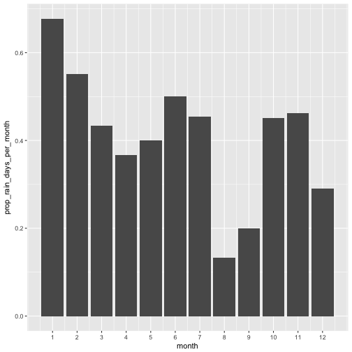
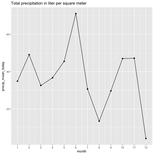
August and September then were quite dry, it appears. Let’s look at the amount of precipitation for comparison.
rain %>%
  group_by(month) %>%
  summarise(precip_mean_today = sum(precip, na.rm = T)) %>%
  ggplot(aes(x = month, y = precip_mean_today)) +
  geom_line() +
  geom_point() +
  scale_x_continuous(breaks = 1:12) +
  labs(title = "Total precipitation in liter per square meter")
For the fun of it, let’s prepare a more nuanced picture.
rain %>%
  ggplot +
  aes(x = date, y = hour, fill = precip) +
  geom_tile() +
  scale_fill_distiller(palette = "Spectral") +
  scale_x_date(date_breaks = "1 month", date_labels = "%b")
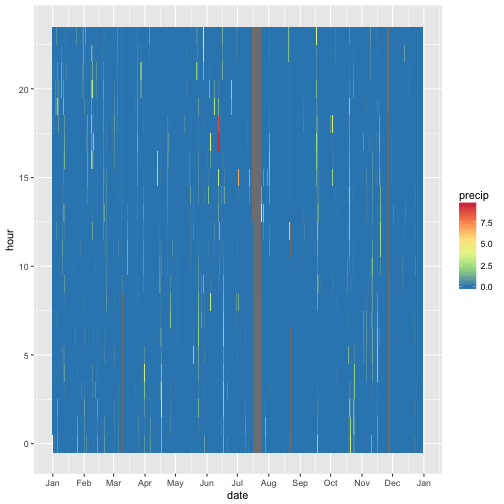
Hey, in June there must have been some heavy raining. Let’s zoom in.
rain %>%
  filter(month == 6) %>%
  ggplot +
  aes(x = date, y = hour, fill = precip) +
  geom_tile() +
  scale_fill_distiller(palette = "Spectral") +
  scale_x_date(date_breaks = "1 day", date_labels = "%d") +
  scale_y_continuous(breaks = c(4, 8, 12, 16, 20, 24))
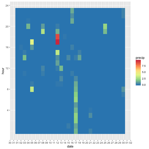
Most of the days in June were dry, but on one day, heave rains occurred on the 12th or 13th in the late afternoon.
rain %>%
  filter(precip > 7)
## # A tibble: 4 x 8
##   precip                  dt   day month  year  hour       date   day_ID
##    <dbl>              <dttm> <int> <dbl> <dbl> <int>     <date>   <time>
## 1    7.4 2016-05-29 21:00:00    29     5  2016    21 2016-05-29 149 days
## 2    9.5 2016-06-12 17:00:00    12     6  2016    17 2016-06-12 163 days
## 3    8.7 2016-06-12 18:00:00    12     6  2016    18 2016-06-12 163 days
## 4    7.2 2016-07-13 15:00:00    13     7  2016    15 2016-07-13 194 days
On June, 12th between 17:00 and 19:00 CEDT, a lot of rain came down in Nuremburg.
Is there a preference for time in terms of precipitation? Maybe it rather rains in the late afternoon in general?
rain %>%
  group_by(hour) %>%
  summarise(precip_mean_per_hour = mean(precip, na.rm = T),
            precip_sd_per_hour = sd(precip, na.rm = T)) %>%
  ggplot +
  aes(x = hour, y = precip_mean_per_hour) +
  geom_line() +
  geom_errorbar(aes(ymin = precip_mean_per_hour - precip_sd_per_hour,
                    ymax = precip_mean_per_hour + precip_sd_per_hour)) +
  geom_point(color = "tomato4")
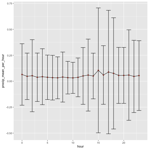
Hm, not much difference between the hours. But the variability seems to differ quite some bit. Would that picture change if we consider only days with precipation?
rain %>%
  filter(precip != 0) %>%
  group_by(hour) %>%
  summarise(precip_mean_per_hour = mean(precip, na.rm = T),
            precip_sd_per_hour = sd(precip, na.rm = T)) %>%
  ggplot +
  aes(x = hour, y = precip_mean_per_hour) +
  geom_line() +
  geom_errorbar(aes(ymin = precip_mean_per_hour - precip_sd_per_hour,
                    ymax = precip_mean_per_hour + precip_sd_per_hour)) +
  geom_point(color = "tomato4")
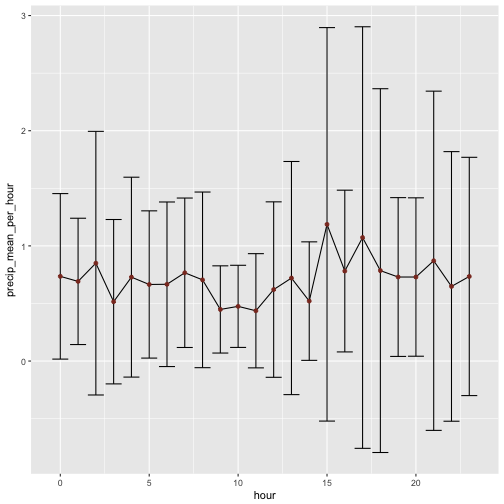
Not too much difference in the overall pattern. But what about if we look at the median and IQR, instead of mean and sd?
rain %>%
  filter(precip != 0) %>%
  group_by(hour) %>%
  summarise(precip_median_per_hour = median(precip, na.rm = T),
            precip_iqr_per_hour = IQR(precip, na.rm = T)) %>%
  ggplot +
  aes(x = hour, y = precip_median_per_hour) +
  geom_line() +
  geom_errorbar(aes(ymin = precip_median_per_hour - precip_iqr_per_hour,
                    ymax = precip_median_per_hour + precip_iqr_per_hour),
                color = "grey60") +
  geom_point(color = "tomato4")
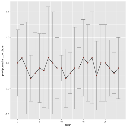
That the pattern breaks down essentially. Not that much difference between the hours left. Maybe 10:00 is rather dry, but that may be sampling errror of this year.