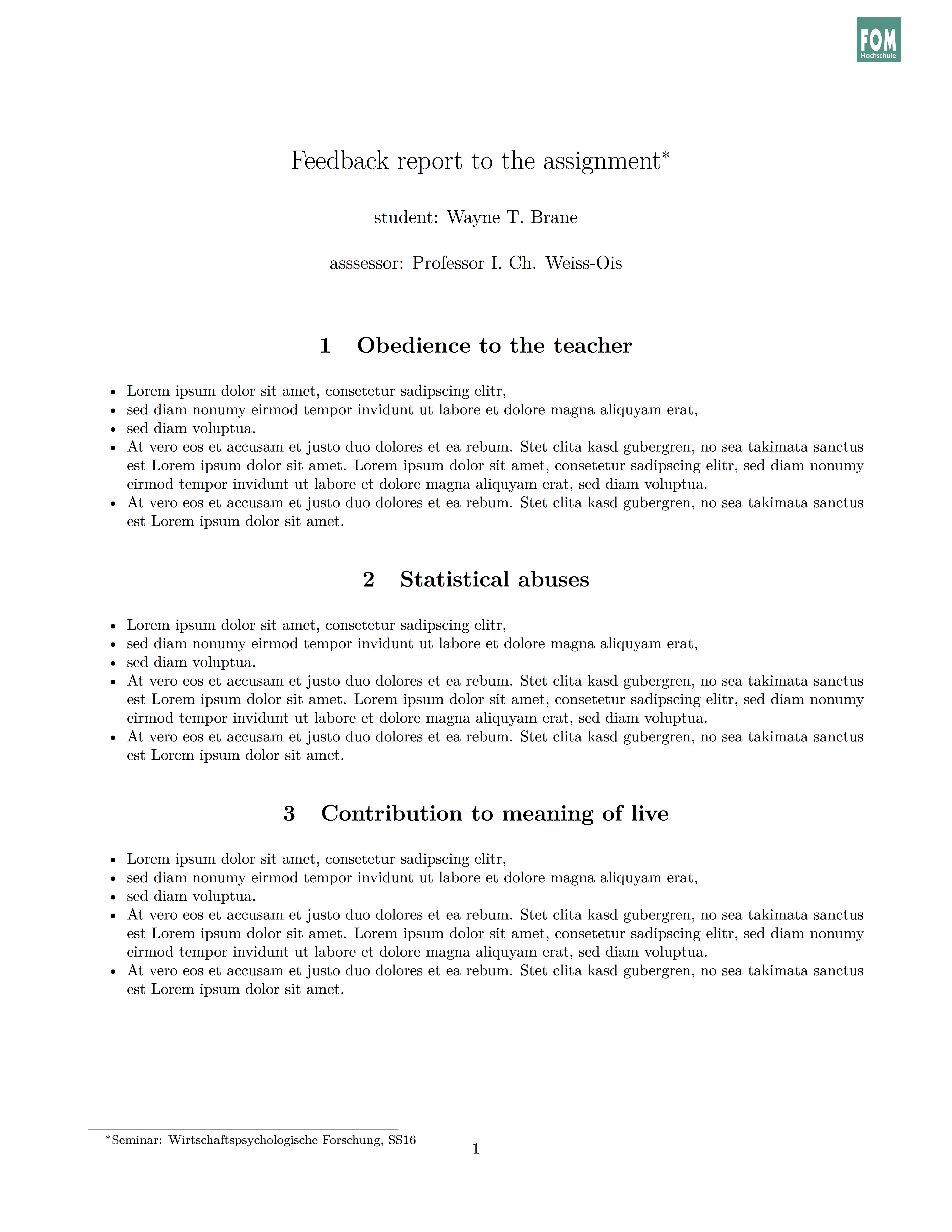
In my role as a teacher, I (have to) write a lot of marking feedback reports. My university provides a website to facilitate the process, that’s great. I have also been writing my reports with Pages, Word, or friends. But somewhat cooler, more attractive, and more reproducible would be using (a markup language such as) Markdown. Basically, that’s easy, but it would be of help to have a template that makes up a nice and nicely formatted report, like this:

Download this pdf file here. Here is the source file. Credit goes to the Pandoc team; I based my template on their’s.

So how to do it?

First and foremorst, write your report using Markdown, and convert it to HTML oder Latex-PDF using Pandoc. Rstudio provides nice introduction, eg., here or here.

Next, tell your Markdown document to use your individual stylesheet, i.e, template. Note that I focus here on PDF output.

---
subtitle: "A general theory ..."
title: "Feedback report to the assignment"
output:
  pdf_document:
    template: template_feedback.latex   
---

You have to put that bit above in the YAML header of your markdown document (right at the top of your document), see the source file for details. And then, you just write your Markdown report in plain English (or whatever language…).

However, where the music actually plays is the latex template, which is being used in the Markdown document (via the YAML header). The idea is that in the Latex file, we define some variables (such as “author” or “title”) which then can be used in the markdown file. Markdown, that is YAML, is able to address those variables defined in the Latex template. In this example, the variables defined include:

  • author
  • title
  • subtitle
  • “thanks to” (I use this field as some “freeride” variable)
  • date

The body (main part) of the onepage example above basically looks like this:


# Obedience to the teacher
- Lorem ipsum dolor sit amet, consetetur sadipscing elitr, 
- sed diam nonumy eirmod tempor invidunt ut labore et dolore magna aliquyam erat, 
- sed diam voluptua. 
...


# Statistical abuses
- Lorem ipsum dolor sit amet, consetetur sadipscing elitr,
...


# Contribution to meaning of live
- Lorem ipsum dolor sit amet, consetetur sadipscing elitr, 
(...)

En plus, the style sheet - being based on Pandoc’s stylesheet - allows for quite a number of more format-based adjustments such as language, geometry of the paper, section-numbering etc. See the excellent Pandoc help for details.

Enjoy!

I just tried to accomplish the following with R: Compute effect sizes for a variable between two groups. Actually, not one numeric variable but many. And compute not only one measure of effect size but several (d, lower/upper CI, CLES,…).

So how to do that?

First, let’s load some data and some (tidyverse and effect size) packages:

knitr::opts_chunk$set(echo = TRUE, cache = FALSE, message = FALSE)
library(purrr)  
library(ggplot2)
library(dplyr)
library(broom)
library(tibble)  

library(compute.es)
data(Fair, package = "Ecdat") # extramarital affairs dataset
glimpse(Fair)
## Observations: 601
## Variables: 9
## $ sex        <fctr> male, female, female, male, male, female, female, ...
## $ age        <dbl> 37, 27, 32, 57, 22, 32, 22, 57, 32, 22, 37, 27, 47,...
## $ ym         <dbl> 10.00, 4.00, 15.00, 15.00, 0.75, 1.50, 0.75, 15.00,...
## $ child      <fctr> no, no, yes, yes, no, no, no, yes, yes, no, yes, y...
## $ religious  <int> 3, 4, 1, 5, 2, 2, 2, 2, 4, 4, 2, 4, 5, 2, 4, 1, 2, ...
## $ education  <dbl> 18, 14, 12, 18, 17, 17, 12, 14, 16, 14, 20, 18, 17,...
## $ occupation <int> 7, 6, 1, 6, 6, 5, 1, 4, 1, 4, 7, 6, 6, 5, 5, 5, 4, ...
## $ rate       <int> 4, 4, 4, 5, 3, 5, 3, 4, 2, 5, 2, 4, 4, 4, 4, 5, 3, ...
## $ nbaffairs  <dbl> 0, 0, 0, 0, 0, 0, 0, 0, 0, 0, 0, 0, 0, 0, 0, 0, 0, ...

Extract the numeric variables:

Fair %>% 
  select_if(is.numeric) %>% names -> Fair_num
Fair_num
## [1] "age"        "ym"         "religious"  "education"  "occupation"
## [6] "rate"       "nbaffairs"

Now suppose we want to compare men and women (people do that all the time). First, we do a t-test for each numeric variable (and save the results):

Fair %>% 
  select(one_of(Fair_num)) %>% 
  map(~t.test(. ~ Fair$sex)) -> Fair_t_test

The resulting variable is a list of t-test-results (each a list again). Let’s have a look at one of the t-test results:

Fair_t_test[[1]]
## 
## 	Welch Two Sample t-test
## 
## data:  . by Fair$sex
## t = -4.7285, df = 575.26, p-value = 2.848e-06
## alternative hypothesis: true difference in means is not equal to 0
## 95 percent confidence interval:
##  -5.014417 -2.071219
## sample estimates:
## mean in group female   mean in group male 
##             30.80159             34.34441

That’s the structure of a t-test result object (one element of Fair_t_test ):

str(Fair_t_test[[1]])
## List of 9
##  $ statistic  : Named num -4.73
##   ..- attr(*, "names")= chr "t"
##  $ parameter  : Named num 575
##   ..- attr(*, "names")= chr "df"
##  $ p.value    : num 2.85e-06
##  $ conf.int   : atomic [1:2] -5.01 -2.07
##   ..- attr(*, "conf.level")= num 0.95
##  $ estimate   : Named num [1:2] 30.8 34.3
##   ..- attr(*, "names")= chr [1:2] "mean in group female" "mean in group male"
##  $ null.value : Named num 0
##   ..- attr(*, "names")= chr "difference in means"
##  $ alternative: chr "two.sided"
##  $ method     : chr "Welch Two Sample t-test"
##  $ data.name  : chr ". by Fair$sex"
##  - attr(*, "class")= chr "htest"

So we see that t-value itself can be accessed with eg., Fair_t_test[[1]]$statistic. The t-value is now fed into a function that computes effect sizes.

Fair_t_test %>% 
  map(~tes(.$statistic,
          n.1 = nrow(filter(Fair, sex == "female")),
          n.2 = nrow(filter(Fair, sex == "male")))) -> Fair_effsize
## Mean Differences ES: 
##  
##  d [ 95 %CI] = -0.39 [ -0.55 , -0.22 ] 
##   var(d) = 0.01 
##   p-value(d) = 0 
##   U3(d) = 34.97 % 
##   CLES(d) = 39.24 % 
##   Cliff's Delta = -0.22 
##  
##  g [ 95 %CI] = -0.39 [ -0.55 , -0.22 ] 
##   var(g) = 0.01 
##   p-value(g) = 0 
##   U3(g) = 34.99 % 
##   CLES(g) = 39.25 % 
##  
##  Correlation ES: 
##  
##  r [ 95 %CI] = 0.19 [ 0.11 , 0.27 ] 
##   var(r) = 0 
##   p-value(r) = 0 
##  
##  z [ 95 %CI] = 0.19 [ 0.11 , 0.27 ] 
##   var(z) = 0 
##   p-value(z) = 0 
##  
##  Odds Ratio ES: 
##  
##  OR [ 95 %CI] = 0.5 [ 0.37 , 0.67 ] 
##   p-value(OR) = 0 
##  
##  Log OR [ 95 %CI] = -0.7 [ -0.99 , -0.41 ] 
##   var(lOR) = 0.02 
##   p-value(Log OR) = 0 
##  
##  Other: 
##  
##  NNT = -11.08 
##  Total N = 601Mean Differences ES: 
##  
##  d [ 95 %CI] = -0.06 [ -0.22 , 0.1 ] 
##   var(d) = 0.01 
##   p-value(d) = 0.46 
##   U3(d) = 47.58 % 
##   CLES(d) = 48.29 % 
##   Cliff's Delta = -0.03 
##  
##  g [ 95 %CI] = -0.06 [ -0.22 , 0.1 ] 
##   var(g) = 0.01 
##   p-value(g) = 0.46 
##   U3(g) = 47.59 % 
##   CLES(g) = 48.29 % 
##  
##  Correlation ES: 
##  
##  r [ 95 %CI] = 0.03 [ -0.05 , 0.11 ] 
##   var(r) = 0 
##   p-value(r) = 0.46 
##  
##  z [ 95 %CI] = 0.03 [ -0.05 , 0.11 ] 
##   var(z) = 0 
##   p-value(z) = 0.46 
##  
##  Odds Ratio ES: 
##  
##  OR [ 95 %CI] = 0.9 [ 0.67 , 1.2 ] 
##   p-value(OR) = 0.46 
##  
##  Log OR [ 95 %CI] = -0.11 [ -0.4 , 0.18 ] 
##   var(lOR) = 0.02 
##   p-value(Log OR) = 0.46 
##  
##  Other: 
##  
##  NNT = -60.47 
##  Total N = 601Mean Differences ES: 
##  
##  d [ 95 %CI] = -0.02 [ -0.18 , 0.15 ] 
##   var(d) = 0.01 
##   p-value(d) = 0.85 
##   U3(d) = 49.39 % 
##   CLES(d) = 49.57 % 
##   Cliff's Delta = -0.01 
##  
##  g [ 95 %CI] = -0.02 [ -0.18 , 0.14 ] 
##   var(g) = 0.01 
##   p-value(g) = 0.85 
##   U3(g) = 49.39 % 
##   CLES(g) = 49.57 % 
##  
##  Correlation ES: 
##  
##  r [ 95 %CI] = 0.01 [ -0.07 , 0.09 ] 
##   var(r) = 0 
##   p-value(r) = 0.85 
##  
##  z [ 95 %CI] = 0.01 [ -0.07 , 0.09 ] 
##   var(z) = 0 
##   p-value(z) = 0.85 
##  
##  Odds Ratio ES: 
##  
##  OR [ 95 %CI] = 0.97 [ 0.73 , 1.3 ] 
##   p-value(OR) = 0.85 
##  
##  Log OR [ 95 %CI] = -0.03 [ -0.32 , 0.26 ] 
##   var(lOR) = 0.02 
##   p-value(Log OR) = 0.85 
##  
##  Other: 
##  
##  NNT = -234.86 
##  Total N = 601Mean Differences ES: 
##  
##  d [ 95 %CI] = -0.86 [ -1.03 , -0.69 ] 
##   var(d) = 0.01 
##   p-value(d) = 0 
##   U3(d) = 19.52 % 
##   CLES(d) = 27.18 % 
##   Cliff's Delta = -0.46 
##  
##  g [ 95 %CI] = -0.86 [ -1.03 , -0.69 ] 
##   var(g) = 0.01 
##   p-value(g) = 0 
##   U3(g) = 19.54 % 
##   CLES(g) = 27.2 % 
##  
##  Correlation ES: 
##  
##  r [ 95 %CI] = 0.39 [ 0.32 , 0.46 ] 
##   var(r) = 0 
##   p-value(r) = 0 
##  
##  z [ 95 %CI] = 0.42 [ 0.34 , 0.5 ] 
##   var(z) = 0 
##   p-value(z) = 0 
##  
##  Odds Ratio ES: 
##  
##  OR [ 95 %CI] = 0.21 [ 0.16 , 0.29 ] 
##   p-value(OR) = 0 
##  
##  Log OR [ 95 %CI] = -1.56 [ -1.86 , -1.25 ] 
##   var(lOR) = 0.02 
##   p-value(Log OR) = 0 
##  
##  Other: 
##  
##  NNT = -6.43 
##  Total N = 601Mean Differences ES: 
##  
##  d [ 95 %CI] = -1.08 [ -1.25 , -0.91 ] 
##   var(d) = 0.01 
##   p-value(d) = 0 
##   U3(d) = 13.95 % 
##   CLES(d) = 22.2 % 
##   Cliff's Delta = -0.56 
##  
##  g [ 95 %CI] = -1.08 [ -1.25 , -0.91 ] 
##   var(g) = 0.01 
##   p-value(g) = 0 
##   U3(g) = 13.98 % 
##   CLES(g) = 22.22 % 
##  
##  Correlation ES: 
##  
##  r [ 95 %CI] = 0.48 [ 0.41 , 0.54 ] 
##   var(r) = 0 
##   p-value(r) = 0 
##  
##  z [ 95 %CI] = 0.52 [ 0.44 , 0.6 ] 
##   var(z) = 0 
##   p-value(z) = 0 
##  
##  Odds Ratio ES: 
##  
##  OR [ 95 %CI] = 0.14 [ 0.1 , 0.19 ] 
##   p-value(OR) = 0 
##  
##  Log OR [ 95 %CI] = -1.96 [ -2.28 , -1.65 ] 
##   var(lOR) = 0.03 
##   p-value(Log OR) = 0 
##  
##  Other: 
##  
##  NNT = -5.79 
##  Total N = 601Mean Differences ES: 
##  
##  d [ 95 %CI] = 0.02 [ -0.15 , 0.18 ] 
##   var(d) = 0.01 
##   p-value(d) = 0.85 
##   U3(d) = 50.6 % 
##   CLES(d) = 50.43 % 
##   Cliff's Delta = 0.01 
##  
##  g [ 95 %CI] = 0.02 [ -0.15 , 0.18 ] 
##   var(g) = 0.01 
##   p-value(g) = 0.85 
##   U3(g) = 50.6 % 
##   CLES(g) = 50.43 % 
##  
##  Correlation ES: 
##  
##  r [ 95 %CI] = 0.01 [ -0.07 , 0.09 ] 
##   var(r) = 0 
##   p-value(r) = 0.85 
##  
##  z [ 95 %CI] = 0.01 [ -0.07 , 0.09 ] 
##   var(z) = 0 
##   p-value(z) = 0.85 
##  
##  Odds Ratio ES: 
##  
##  OR [ 95 %CI] = 1.03 [ 0.77 , 1.37 ] 
##   p-value(OR) = 0.85 
##  
##  Log OR [ 95 %CI] = 0.03 [ -0.26 , 0.32 ] 
##   var(lOR) = 0.02 
##   p-value(Log OR) = 0.85 
##  
##  Other: 
##  
##  NNT = 235.02 
##  Total N = 601Mean Differences ES: 
##  
##  d [ 95 %CI] = -0.02 [ -0.18 , 0.14 ] 
##   var(d) = 0.01 
##   p-value(d) = 0.77 
##   U3(d) = 49.06 % 
##   CLES(d) = 49.34 % 
##   Cliff's Delta = -0.01 
##  
##  g [ 95 %CI] = -0.02 [ -0.18 , 0.14 ] 
##   var(g) = 0.01 
##   p-value(g) = 0.77 
##   U3(g) = 49.07 % 
##   CLES(g) = 49.34 % 
##  
##  Correlation ES: 
##  
##  r [ 95 %CI] = 0.01 [ -0.07 , 0.09 ] 
##   var(r) = 0 
##   p-value(r) = 0.77 
##  
##  z [ 95 %CI] = 0.01 [ -0.07 , 0.09 ] 
##   var(z) = 0 
##   p-value(z) = 0.77 
##  
##  Odds Ratio ES: 
##  
##  OR [ 95 %CI] = 0.96 [ 0.72 , 1.28 ] 
##   p-value(OR) = 0.77 
##  
##  Log OR [ 95 %CI] = -0.04 [ -0.33 , 0.25 ] 
##   var(lOR) = 0.02 
##   p-value(Log OR) = 0.77 
##  
##  Other: 
##  
##  NNT = -153.72 
##  Total N = 601

The resulting object (Fair_effsize) is a list where each list element is the output of the tes function. Let’s have a look at one of these list elements:

Fair_effsize[[1]]
##   N.total n.1 n.2     d var.d   l.d   u.d  U3.d  cl.d cliffs.d pval.d
## t     601 315 286 -0.39  0.01 -0.55 -0.22 34.97 39.24    -0.22      0
##       g var.g   l.g   u.g  U3.g  cl.g pval.g    r var.r  l.r  u.r pval.r
## t -0.39  0.01 -0.55 -0.22 34.99 39.25      0 0.19     0 0.11 0.27      0
##   fisher.z var.z  l.z  u.z  OR l.or u.or pval.or  lOR l.lor u.lor pval.lor
## t     0.19     0 0.11 0.27 0.5 0.37 0.67       0 -0.7 -0.99 -0.41        0
##      NNT
## t -11.08
str(Fair_effsize[[1]])
## 'data.frame':	1 obs. of  36 variables:
##  $ N.total : num 601
##  $ n.1     : num 315
##  $ n.2     : num 286
##  $ d       : num -0.39
##  $ var.d   : num 0.01
##  $ l.d     : num -0.55
##  $ u.d     : num -0.22
##  $ U3.d    : num 35
##  $ cl.d    : num 39.2
##  $ cliffs.d: num -0.22
##  $ pval.d  : num 0
##  $ g       : num -0.39
##  $ var.g   : num 0.01
##  $ l.g     : num -0.55
##  $ u.g     : num -0.22
##  $ U3.g    : num 35
##  $ cl.g    : num 39.2
##  $ pval.g  : num 0
##  $ r       : num 0.19
##  $ var.r   : num 0
##  $ l.r     : num 0.11
##  $ u.r     : num 0.27
##  $ pval.r  : num 0
##  $ fisher.z: num 0.19
##  $ var.z   : num 0
##  $ l.z     : num 0.11
##  $ u.z     : num 0.27
##  $ OR      : num 0.5
##  $ l.or    : num 0.37
##  $ u.or    : num 0.67
##  $ pval.or : num 0
##  $ lOR     : num -0.7
##  $ l.lor   : num -0.99
##  $ u.lor   : num -0.41
##  $ pval.lor: num 0
##  $ NNT     : num -11.1

The element itself is a data frame with n=1 and p=36. So we could nicely row-bind these 36 rows into one data frame. How to do that?

Fair_effsize %>% 
  map( ~do.call(rbind, .)) %>% 
  as.data.frame -> Fair_effsize_df

head(Fair_effsize_df)
##            age     ym religious education occupation   rate nbaffairs
## N.total 601.00 601.00    601.00    601.00     601.00 601.00    601.00
## n.1     315.00 315.00    315.00    315.00     315.00 315.00    315.00
## n.2     286.00 286.00    286.00    286.00     286.00 286.00    286.00
## d        -0.39  -0.06     -0.02     -0.86      -1.08   0.02     -0.02
## var.d     0.01   0.01      0.01      0.01       0.01   0.01      0.01
## l.d      -0.55  -0.22     -0.18     -1.03      -1.25  -0.15     -0.18

What we did here is:

  1. Take each list element and then… (that was map)
  2. bind these elements row-wise together, ie,. “underneath” each other (rbind). do.call is only a helper that allows to hand over to rbind a bunch of rows.
  3. Then convert this element, still a list, to a data frame (not much changes in effect)

Finally, let’s convert the row names to a column:

Fair_effsize_df %>% 
  rownames_to_column -> Fair_effsize_df

head(Fair_effsize_df)
##   rowname    age     ym religious education occupation   rate nbaffairs
## 1 N.total 601.00 601.00    601.00    601.00     601.00 601.00    601.00
## 2     n.1 315.00 315.00    315.00    315.00     315.00 315.00    315.00
## 3     n.2 286.00 286.00    286.00    286.00     286.00 286.00    286.00
## 4       d  -0.39  -0.06     -0.02     -0.86      -1.08   0.02     -0.02
## 5   var.d   0.01   0.01      0.01      0.01       0.01   0.01      0.01
## 6     l.d  -0.55  -0.22     -0.18     -1.03      -1.25  -0.15     -0.18

A bit of a ride, but we got there!

And I am sure, better ways are out there. Let me know!

A frequent task in data analysis is to get a summary of a bunch of variables. Often, graphical summaries (diagrams) are wanted. However, at times numerical summaries are in order. How to get that in R? That’s the question of the present post.

Of course, there are several ways. One way, using purrr, is the following. I liked it quite a bit that’s why I am showing it here.

First, let’s load some data and some packages we will make use of.

data(Affairs, package = "AER")

library(purrr)
library(dplyr)
library(broom)

Define two helper functions we will need later on:

add_na_col <- function(x){
  mutate(x, na = 0)
}

has_n_col <- function(x, n = 6){
  return(ncol(x) == n)
}

Set one value to NA for illustration purposes:

Affairs$affairs[1] <- NA  # one NA for illustrative purposes

Now comes the show:

Affairs %>%
  select_if(is.numeric)  %>%
  map(~tidy(summary(.x))) %>%  # compute tidy summary of each var
  map_if(., has_n_col, add_na_col) %>%   # add na-col if missing
  do.call(rbind, .) -> Affairs_summary  # bind list elements into df

Affairs_summary
##               minimum q1 median   mean    q3 maximum na
## affairs         0.000  0      0  1.458  0.25      12  1
## age            17.500 27     32 32.490 37.00      57  0
## yearsmarried    0.125  4      7  8.178 15.00      15  0
## religiousness   1.000  2      3  3.116  4.00       5  0
## education       9.000 14     16 16.170 18.00      20  0
## occupation      1.000  3      5  4.195  6.00       7  0
## rating          1.000  3      4  3.932  5.00       5  0

What we did was:

  1. Get the Affairs data, and select the numeric columns
  2. Map the summary function to each column, and tidy up each column. We will get a list of tidy summaries.
  3. If a list element has 6 elements (or columns, because we want to end up with a data frame), then we know there is no NA-column. In this case, add_na_col, else not. That’s what the map_if bit does.
  4. Lastly, bind the list elements row wise. To that end, give a bag of summary-elements to rbind by help of do.call.

Instead of purr::map, a more familiar approach would have been this:

Affairs %>%
  dplyr::select_if(is.numeric)  %>%
  lapply(., function(x) tidy(summary(x)))  # compute tidy summary of each var
## $affairs
##   minimum q1 median  mean   q3 maximum na
## 1       0  0      0 1.458 0.25      12  1
## 
## $age
##   minimum q1 median  mean q3 maximum
## 1    17.5 27     32 32.49 37      57
## 
## $yearsmarried
##   minimum q1 median  mean q3 maximum
## 1   0.125  4      7 8.178 15      15
## 
## $religiousness
##   minimum q1 median  mean q3 maximum
## 1       1  2      3 3.116  4       5
## 
## $education
##   minimum q1 median  mean q3 maximum
## 1       9 14     16 16.17 18      20
## 
## $occupation
##   minimum q1 median  mean q3 maximum
## 1       1  3      5 4.195  6       7
## 
## $rating
##   minimum q1 median  mean q3 maximum
## 1       1  3      4 3.932  5       5

And, finally, a quite nice formatting tool for html tables is DT:datatable (output not shown):

library(DT)
datatable(Affairs_summary)

Although this approach may not work in each environment, particularly not with knitr (as far as I know of).

That’s why an alternative html table approach is used:

library(htmlTable)

htmlTable(Affairs_summary)
minimum q1 median mean q3 maximum na
affairs 0 0 0 1.458 0.25 12 1
age 17.5 27 32 32.49 37 57 0
yearsmarried 0.125 4 7 8.178 15 15 0
religiousness 1 2 3 3.116 4 5 0
education 9 14 16 16.17 18 20 0
occupation 1 3 5 4.195 6 7 0
rating 1 3 4 3.932 5 5 0

EDIT based on comments/ suggeestions from @JonoCarroll Disqus profile and @tjmahr twitter profile. See below (last step; look for “EDIT”).

Thanks for the input! :thumbsup:

reading time: 10 min.

Hadley Wickham’s purrr has given a new look at handling data structures to the typical R user (some reasoning suggests that average users doesn’t exist, but that’s a different story).

I just tried the following with purrr:

  • Meditate about the running a simple regression, FWIW
  • Take a dataframe with candidate predictors and an outcome
  • Throw one predictor at a time into the regression, where the outcome variable remains the same (i.,e multiple simple regressions (one predictor) where the predictor is changed at each run but the outcome remains the same)
  • tidy up the resulting $R^2$ in some nice format

I found that purrr does the job nicely, and it’s quite instructive to see purrrat work, I think. That’s why I wrote it up in this short post:

library(purrr)  
library(ggplot2)
library(dplyr)
library(broom)
library(knitr)  # for kable
data(Fair, package = "Ecdat") # extramarital affairs dataset
glimpse(Fair)
## Observations: 601
## Variables: 9
## $ sex        <fctr> male, female, female, male, male, female, female, ...
## $ age        <dbl> 37, 27, 32, 57, 22, 32, 22, 57, 32, 22, 37, 27, 47,...
## $ ym         <dbl> 10.00, 4.00, 15.00, 15.00, 0.75, 1.50, 0.75, 15.00,...
## $ child      <fctr> no, no, yes, yes, no, no, no, yes, yes, no, yes, y...
## $ religious  <int> 3, 4, 1, 5, 2, 2, 2, 2, 4, 4, 2, 4, 5, 2, 4, 1, 2, ...
## $ education  <dbl> 18, 14, 12, 18, 17, 17, 12, 14, 16, 14, 20, 18, 17,...
## $ occupation <int> 7, 6, 1, 6, 6, 5, 1, 4, 1, 4, 7, 6, 6, 5, 5, 5, 4, ...
## $ rate       <int> 4, 4, 4, 5, 3, 5, 3, 4, 2, 5, 2, 4, 4, 4, 4, 5, 3, ...
## $ nbaffairs  <dbl> 0, 0, 0, 0, 0, 0, 0, 0, 0, 0, 0, 0, 0, 0, 0, 0, 0, ...
Fair %>% 
  dplyr::select(-nbaffairs) %>%  # exclude outcome, leave only predictors 
  map(~lm(Fair$nbaffairs ~ .x, data = Fair)) %>% 
  map(summary) %>% 
  map_dbl("r.squared") %>% 
  tidy %>% 
  dplyr::arrange(desc(x)) %>% 
  rename(r.squared = x) -> r2s

kable(r2s)
names r.squared
rate 0.0781272
ym 0.0349098
religious 0.0208806
child 0.0108181
age 0.0090701
occupation 0.0024613
sex 0.0001377
education 0.0000059

Ok, that appears to be the list of the $R^2$ for each simple (one-predictor) regression we have run.

Let’s do a quick sense check with the standard way:

lm1 <- lm(nbaffairs ~ rate, data = Fair)

summary(lm1)
## 
## Call:
## lm(formula = nbaffairs ~ rate, data = Fair)
## 
## Residuals:
##     Min      1Q  Median      3Q     Max 
## -3.9063 -1.3989 -0.5631 -0.5631 11.4369 
## 
## Coefficients:
##             Estimate Std. Error t value Pr(>|t|)    
## (Intercept)   4.7421     0.4790   9.900   <2e-16 ***
## rate         -0.8358     0.1173  -7.125    3e-12 ***
## ---
## Signif. codes:  0 '***' 0.001 '**' 0.01 '*' 0.05 '.' 0.1 ' ' 1
## 
## Residual standard error: 3.17 on 599 degrees of freedom
## Multiple R-squared:  0.07813,	Adjusted R-squared:  0.07659 
## F-statistic: 50.76 on 1 and 599 DF,  p-value: 3.002e-12
summary(lm1)$r.squared
## [1] 0.07812718
summary(lm1)$coefficients[2, 4]  #p.value
## [1] 3.002385e-12

Seems to work. To get details of the object summary(lm1), use str(summary(lm1)).

How many did we run? Just the number of columns minus one (the outcome variable).

ncol(Fair)-1
## [1] 8

FWIW, let’s plot the resulting values (and sort the predictors by descending values).

ggplot(r2s, aes(x = reorder(names, r.squared), y = r.squared)) + 
  geom_point(size = 5, color = "red") +
  ylab(expression(R^{2})) +
  xlab("predictors") +
  ggtitle("Explained variance per predictor from simple regressions")

plot of chunk unnamed-chunk-4

Wait, one more thing. Suppose we are not only interested in \(R^2\), but in the p-values (OMG). How to get both values from purrr?.


EDIT (the following part has changed)


Thanks for comments from @JonoCarroll Disqus profile and @tjmahr twitter profile, the last step - extracting the p-values - is now changed, and I think improved.

Fair %>% 
  dplyr::select(-nbaffairs) %>%  # exclude outcome, leave only predictors 
  map(~lm(Fair$nbaffairs ~ .x, data = Fair)) %>% 
  map(summary) %>% 
  map(broom::tidy) %>% 
  map_df("p.value")  %>% 
  round(3) %>% 
  mutate(variable = c("intercept", "predictor")) -> ps
library(htmlTable)

htmlTable(ps)
sex age ym child religious education occupation rate variable
1 0 0.465 0.019 0 0 0.1 0.002 0 intercept
2 0.774 0.02 0 0.011 0 0.952 0.225 0 predictor

So what I did above basically is:

  • Run a linear model on each predictor
  • Get a summary of each model
  • Tidy (with broom) each summary
  • Get the sublist (column) p.value from each list (model), and save the result as a data frame

To get a whole bunch of relevant statistics, you can use glance:

Fair %>% 
  dplyr::select(-nbaffairs) %>%  # exclude outcome, leave only predictors 
  map( ~lm(Fair$nbaffairs ~ .x, data = Fair)) %>% 
  map(summary) %>% 
  map_df(glance) %>% 
  round(3)
##   r.squared adj.r.squared sigma statistic p.value df
## 1     0.000        -0.002 3.301     0.083   0.774  2
## 2     0.009         0.007 3.287     5.483   0.020  2
## 3     0.035         0.033 3.243    21.667   0.000  2
## 4     0.011         0.009 3.284     6.551   0.011  2
## 5     0.021         0.019 3.267    12.774   0.000  2
## 6     0.000        -0.002 3.302     0.004   0.952  2
## 7     0.002         0.001 3.297     1.478   0.225  2
## 8     0.078         0.077 3.170    50.764   0.000  2

Thanks for comments from @JonoCarroll Disqus profile and @tjmahr twitter profile, the last step - extracting the p-values - is now changed, and I think improved.

Hadley Wickham’s purrr has given a new look at handling data structures to the typical R user (some reasoning suggests that average users don’t exist, but that’s a different story).

I just tried the following with purrr:

  • Meditate about the running a simple regression, FWIW
  • Take a dataframe with candidate predictors and an outcome
  • Throw one predictor at a time into the regression, where the outcome variable remains the same (i.,e multiple simple regressions (one predictor) where the predictor is changed at each run but the outcome remains the same)
  • tidy up the resulting \(R^2\) in some nice format.

I found that purrr does the job nicely, and it’s quite instructive, I think. That’s why I wrote it up in this short post:

library(purrr)  
library(ggplot2)
library(dplyr)
library(broom)
library(knitr)  # for kable
data(Fair, package = "Ecdat") # extramarital affairs dataset
glimpse(Fair)
## Observations: 601
## Variables: 9
## $ sex        <fctr> male, female, female, male, male, female, female, ...
## $ age        <dbl> 37, 27, 32, 57, 22, 32, 22, 57, 32, 22, 37, 27, 47,...
## $ ym         <dbl> 10.00, 4.00, 15.00, 15.00, 0.75, 1.50, 0.75, 15.00,...
## $ child      <fctr> no, no, yes, yes, no, no, no, yes, yes, no, yes, y...
## $ religious  <int> 3, 4, 1, 5, 2, 2, 2, 2, 4, 4, 2, 4, 5, 2, 4, 1, 2, ...
## $ education  <dbl> 18, 14, 12, 18, 17, 17, 12, 14, 16, 14, 20, 18, 17,...
## $ occupation <int> 7, 6, 1, 6, 6, 5, 1, 4, 1, 4, 7, 6, 6, 5, 5, 5, 4, ...
## $ rate       <int> 4, 4, 4, 5, 3, 5, 3, 4, 2, 5, 2, 4, 4, 4, 4, 5, 3, ...
## $ nbaffairs  <dbl> 0, 0, 0, 0, 0, 0, 0, 0, 0, 0, 0, 0, 0, 0, 0, 0, 0, ...
Fair %>% 
  dplyr::select(-nbaffairs) %>%  # exclude outcome, leave only predictors 
  map(~lm(Fair$nbaffairs ~ .x, data = Fair)) %>% 
  map(summary) %>% 
  map_dbl("r.squared") %>% 
  tidy %>% 
  dplyr::arrange(desc(x)) %>% 
  rename(r.squared = x) -> r2s

kable(r2s)
names r.squared
rate 0.0781272
ym 0.0349098
religious 0.0208806
child 0.0108181
age 0.0090701
occupation 0.0024613
sex 0.0001377
education 0.0000059

Ok, that appears to be the list of the \(R^{2}\) for each simple (one-predictor) regression we have run.

Let’s do a quick sense check with the standard way:

lm1 <- lm(nbaffairs ~ rate, data = Fair)

summary(lm1)
## 
## Call:
## lm(formula = nbaffairs ~ rate, data = Fair)
## 
## Residuals:
##     Min      1Q  Median      3Q     Max 
## -3.9063 -1.3989 -0.5631 -0.5631 11.4369 
## 
## Coefficients:
##             Estimate Std. Error t value Pr(>|t|)    
## (Intercept)   4.7421     0.4790   9.900   <2e-16 ***
## rate         -0.8358     0.1173  -7.125    3e-12 ***
## ---
## Signif. codes:  0 '***' 0.001 '**' 0.01 '*' 0.05 '.' 0.1 ' ' 1
## 
## Residual standard error: 3.17 on 599 degrees of freedom
## Multiple R-squared:  0.07813,	Adjusted R-squared:  0.07659 
## F-statistic: 50.76 on 1 and 599 DF,  p-value: 3.002e-12
summary(lm1)$r.squared
## [1] 0.07812718
summary(lm1)$coefficients[2, 4]  #p.value
## [1] 3.002385e-12

Seems to work. To get details of the object summary(lm1), use str(summary(lm1)).

How many did we run? Just the number of columns minus one (the outcome variable).

ncol(Fair)-1
## [1] 8

FWIW, let’s plot the resulting values (and sort the predictors by descending values).

ggplot(r2s, aes(x = reorder(names, r.squared), y = r.squared)) + 
  geom_point(size = 5, color = "red") +
  ylab(expression(R^{2})) +
  xlab("predictors") +
  ggtitle("Explained variance per predictor from simple regressions")

Wait, one more thing. Suppose we are not only interested in \(R^{2}\), but in the p-values (OMG). How to get both values from purrr?.

library(magrittr)

Fair %>% 
  dplyr::select(-nbaffairs) %>%  # exclude outcome, leave only predictors 
  map(~lm(Fair$nbaffairs ~ .x, data = Fair)) %>% 
  map(summary) %>% 
  map(c("coefficients")) %>% 
  map_dbl(8)  %>% # 8th element is the p-value 
  tidy %>% 
  dplyr::arrange(desc(x)) %>% 
  rename(p.value = x) -> ps
  
  
kable(ps)
names p.value
education 0.9524501
sex 0.7740138
occupation 0.2245709
age 0.0195320
child 0.0107275
religious 0.0003797
ym 0.0000040
rate 0.0000000

Extracting the p-value by map_dbl(8) is surely far from perfect. Any ideas how to better get the value out of this numeric 2*4 matrix? Thoughts are welcome!