On a recent psychology conference I had the impression that psychologists keep preferring to show mean values, but appear less interested in more detailled plots such as the boxplot. Plots like the boxplot are richer in information, but not more difficult to perceive.

For those who would like to have an easy starter on how to visualize more informative plots (more than mean bars), here is a suggestion:

# install.pacakges("Ecdat")
library(Ecdat)  # dataset on extramarital affairs
data(Fair)
str(Fair)
## 'data.frame':	601 obs. of  9 variables:
##  $ sex       : Factor w/ 2 levels "female","male": 2 1 1 2 2 1 1 2 1 2 ...
##  $ age       : num  37 27 32 57 22 32 22 57 32 22 ...
##  $ ym        : num  10 4 15 15 0.75 1.5 0.75 15 15 1.5 ...
##  $ child     : Factor w/ 2 levels "no","yes": 1 1 2 2 1 1 1 2 2 1 ...
##  $ religious : int  3 4 1 5 2 2 2 2 4 4 ...
##  $ education : num  18 14 12 18 17 17 12 14 16 14 ...
##  $ occupation: int  7 6 1 6 6 5 1 4 1 4 ...
##  $ rate      : int  4 4 4 5 3 5 3 4 2 5 ...
##  $ nbaffairs : num  0 0 0 0 0 0 0 0 0 0 ...
library(ggplot2)
library(dplyr)

Fair %>% 
  filter(nbaffairs != 0) %>% 
  ggplot(aes(x = sex, y = nbaffairs)) +
  ggtitle("Difference in extramarital affairs between sexes") +
  geom_boxplot() +
  geom_jitter(alpha = .5, color = "firebrick") +
  theme_minimal()

plot of chunk unnamed-chunk-1

As can be seen, the distribution information reveals some more insight than bare means: There appear to be three distinct groups of “side lookers” (persons having extramarital relations).

This would not come out if looking at means only:

Fair %>% 
  na.omit() %>% 
  group_by(sex) %>% 
  summarise(mean_affair_by_sex = mean(nbaffairs)) %>% 
  ggplot(aes(x= sex, y = mean_affair_by_sex)) +
  geom_bar(stat = "identity") +
  ggtitle("Mean value difference in extramarital affairs between sexes")

plot of chunk unnamed-chunk-2

I just attended the biannual conference of the German society of psychology (DPGs) in Leipzig; open science was a central, albeit not undisputed topic; a lot of interesting related twitter discussion.

image source: Felix Schönbrodt

Interestingly, a strong voice of German scientiests uttered their concerns about being scooped if/when sharing their data (during the official meeting of the society). This being said (sad), the German research foundation (DFG) has updated its guidelines now stressing (more strongly) that publicly funded projects should share their data, with the rationale that the data do not belong to the individual scientiest but to the public, as the public funded it (I find that convincing). Finally, Brian Nosek had a key note talk, where he vividly argued in favor of open science; I found the talk very inspiring.

Anyway, I do not want to discuss the “why” and “if” but rather the “how” in this post, giving some recommendations. Or more precisely, what I personally do at the moment for living up to open science. The following list is by no means innovative, impressive, it just presents my current thinking and doing:

  • Share you code, e.g., on Github
  • Spread the word (blog your thoughts), Github and Jekyll provide a cool tool
  • Sign the (or one of the) research transparency initiatives for reviewers, and live up to it
  • Publish your data, e.g., on Open Science Framework (OSF)
  • Publish a data paper, e.g., here, and get a citable paper out of in it, including a doi
  • Checkout whether your pay-walled journal accepts preprint/postprint open access (many do!) (BTW: Here’s a blog post explaining differences between preprints and postprints, and what your rights are)
  • Put your preprint/postprint on a repository, eg., OSF or SocArXiv
  • If you are editor or faculty head: promote open science in your environment
  • Preregister your study, eg. on OSF
  • Learn more about good data (management/analysis) practices, e.g, on OSF
  • Connect on social media, e.g, Twitter hashtag #openscience
  • Consider becoming an ambassador of open science at COS

Peronally, I put my code on Github, and my data and preprints to OSF (and other stuff, such as presentations, too). And I blog and twitter on that (among other topics).

The list above is surely not exhaustive, nor it is definitely mandatory to submit to each item. I am to still learning and getting more into it.

I think we should consider that it may well be that our research results are mostly false, see Paul Meehls seminal paper(s), and of course the results of the Reproducibilty Project Psychology, among many others sources.

Hopefully, we will not drift astray in emotional discussions on “research parasites”, “methodological terrorists”, or “cyberbullies”, but focus on what is constructive for our field. One could argue that the only question that counts is “How do I contribute?”.


YADCSDA in German language.


In dieser Fallstudie (YACSDA: Yet another case study of data analysis) wird der Datensatz TopGear analysiert, vor allem mit grafischen Mitteln. Es handelt sich weniger um einen “Rundumschlag” zur Beantwortung aller möglichen interessanten Fragen (oder zur Demonstration aller möglichen Analysewerkzeuge), sondern eher um einen Einblick zu einfachen explorativen Verfahren.

library(robustHD)
## Loading required package: perry
## Loading required package: parallel
## Loading required package: robustbase
data(TopGear)  # Daten aus Package laden
library(tidyverse)

Numerischer Überblick

glimpse(TopGear)
## Observations: 297
## Variables: 32
## $ Maker              <fctr> Alfa Romeo, Alfa Romeo, Aston Martin, Asto...
## $ Model              <fctr> Giulietta, MiTo, Cygnet, DB9, DB9 Volante,...
## $ Type               <fctr> Giulietta 1.6 JTDM-2 105 Veloce 5d, MiTo 1...
## $ Fuel               <fctr> Diesel, Petrol, Petrol, Petrol, Petrol, Pe...
## $ Price              <dbl> 21250, 15155, 30995, 131995, 141995, 396000...
## $ Cylinders          <dbl> 4, 4, 4, 12, 12, 12, 12, 8, 8, 4, 4, 4, 4, ...
## $ Displacement       <dbl> 1598, 1368, 1329, 5935, 5935, 5935, 5935, 4...
## $ DriveWheel         <fctr> Front, Front, Front, Rear, Rear, Rear, Rea...
## $ BHP                <dbl> 105, 105, 98, 517, 517, 510, 573, 420, 420,...
## $ Torque             <dbl> 236, 95, 92, 457, 457, 420, 457, 346, 346, ...
## $ Acceleration       <dbl> 11.3, 10.7, 11.8, 4.6, 4.6, 4.2, 4.1, 4.7, ...
## $ TopSpeed           <dbl> 115, 116, 106, 183, 183, 190, 183, 180, 180...
## $ MPG                <dbl> 64, 49, 56, 19, 19, 17, 19, 20, 20, 55, 54,...
## $ Weight             <dbl> 1385, 1090, 988, 1785, 1890, 1680, 1739, 16...
## $ Length             <dbl> 4351, 4063, 3078, 4720, 4720, 4385, 4720, 4...
## $ Width              <dbl> 1798, 1720, 1680, NA, NA, 1865, 1910, 1865,...
## $ Height             <dbl> 1465, 1446, 1500, 1282, 1282, 1250, 1294, 1...
## $ AdaptiveHeadlights <fctr> optional, optional, no, standard, standard...
## $ AdjustableSteering <fctr> standard, standard, standard, standard, st...
## $ AlarmSystem        <fctr> standard, standard, no/optional, no/option...
## $ Automatic          <fctr> no, no, optional, standard, standard, no, ...
## $ Bluetooth          <fctr> standard, standard, standard, standard, st...
## $ ClimateControl     <fctr> standard, optional, standard, standard, st...
## $ CruiseControl      <fctr> standard, standard, standard, standard, st...
## $ ElectricSeats      <fctr> optional, no, no, standard, standard, stan...
## $ Leather            <fctr> optional, optional, no, standard, standard...
## $ ParkingSensors     <fctr> optional, standard, no, standard, standard...
## $ PowerSteering      <fctr> standard, standard, standard, standard, st...
## $ SatNav             <fctr> optional, optional, standard, standard, st...
## $ ESP                <fctr> standard, standard, standard, standard, st...
## $ Verdict            <dbl> 6, 5, 7, 7, 7, 7, 7, 8, 7, 6, 7, 6, 5, 7, 6...
## $ Origin             <fctr> Europe, Europe, Europe, Europe, Europe, Eu...
summary(TopGear)
##            Maker                      Model    
##  Mercedes-Benz: 19   Roadster            :  2  
##  Audi         : 18   1 Series            :  1  
##  BMW          : 18   1 Series Convertible:  1  
##  Vauxhall     : 17   1 Series Coupe      :  1  
##  Volkswagen   : 15   107                 :  1  
##  Toyota       : 11   207 CC              :  1  
##  (Other)      :199   (Other)             :290  
##                             Type         Fuel         Price        
##  107 1.0 68 Active 5d         :  1   Diesel:112   Min.   :   6950  
##  118d SE 5d                   :  1   Petrol:180   1st Qu.:  18910  
##  120d SE Convertible 2d       :  1   NA's  :  5   Median :  26495  
##  120i M Sport Coupe 2d        :  1                Mean   :  50784  
##  12C 3.8 V8 TT 625 Standard 2d:  1                3rd Qu.:  44195  
##  207 CC 1.6 VTi 120 GT 2d     :  1                Max.   :1139985  
##  (Other)                      :291                                 
##    Cylinders       Displacement  DriveWheel       BHP       
##  Min.   : 0.000   Min.   : 647   4WD  : 67   Min.   : 17.0  
##  1st Qu.: 4.000   1st Qu.:1560   Front:147   1st Qu.:112.0  
##  Median : 4.000   Median :1995   Rear : 78   Median :160.0  
##  Mean   : 5.055   Mean   :2504   NA's :  5   Mean   :218.3  
##  3rd Qu.: 6.000   3rd Qu.:2988               3rd Qu.:258.0  
##  Max.   :16.000   Max.   :7993               Max.   :987.0  
##  NA's   :4        NA's   :9                  NA's   :4      
##      Torque       Acceleration       TopSpeed          MPG        
##  Min.   : 42.0   Min.   : 0.000   Min.   : 50.0   Min.   : 10.00  
##  1st Qu.:151.0   1st Qu.: 5.900   1st Qu.:112.0   1st Qu.: 34.00  
##  Median :236.0   Median : 9.100   Median :126.0   Median : 47.00  
##  Mean   :255.4   Mean   : 8.839   Mean   :132.7   Mean   : 48.11  
##  3rd Qu.:324.0   3rd Qu.:11.400   3rd Qu.:151.0   3rd Qu.: 57.00  
##  Max.   :922.0   Max.   :16.900   Max.   :252.0   Max.   :470.00  
##  NA's   :4                        NA's   :4       NA's   :12      
##      Weight         Length         Width          Height    
##  Min.   : 210   Min.   :2337   Min.   :1237   Min.   :1115  
##  1st Qu.:1244   1st Qu.:4157   1st Qu.:1760   1st Qu.:1421  
##  Median :1494   Median :4464   Median :1815   Median :1484  
##  Mean   :1536   Mean   :4427   Mean   :1811   Mean   :1510  
##  3rd Qu.:1774   3rd Qu.:4766   3rd Qu.:1877   3rd Qu.:1610  
##  Max.   :2705   Max.   :5612   Max.   :2073   Max.   :1951  
##  NA's   :33     NA's   :11     NA's   :16     NA's   :11    
##  AdaptiveHeadlights AdjustableSteering      AlarmSystem     Automatic  
##  no      :137       no      : 73       no/optional:112   no      :111  
##  optional: 28       standard:224       standard   :185   optional: 87  
##  standard:132                                            standard: 99  
##                                                                        
##                                                                        
##                                                                        
##                                                                        
##     Bluetooth    ClimateControl  CruiseControl  ElectricSeats
##  no      : 55   no      : 83    no      : 87   no      :187  
##  optional: 46   optional: 35    optional: 35   optional: 35  
##  standard:196   standard:179    standard:175   standard: 75  
##                                                              
##                                                              
##                                                              
##                                                              
##      Leather     ParkingSensors  PowerSteering      SatNav   
##  no      :124   no      : 72    no      : 27   no      : 86  
##  optional: 56   optional: 61    standard:270   optional:116  
##  standard:117   standard:164                   standard: 95  
##                                                              
##                                                              
##                                                              
##                                                              
##        ESP         Verdict          Origin   
##  no      : 24   Min.   : 1.000   Asia  : 74  
##  optional: 16   1st Qu.: 5.000   Europe:198  
##  standard:257   Median : 7.000   USA   : 25  
##                 Mean   : 6.339               
##                 3rd Qu.: 7.000               
##                 Max.   :10.000               
##                 NA's   :2

Wie verteilen sich die Preise?

Die Funktion qplot() ist ein einfacher Weg, um Daten zu visualisieren.

qplot(data = TopGear, x = Price, geom = "histogram")
## `stat_bin()` using `bins = 30`. Pick better value with `binwidth`.

plot of chunk unnamed-chunk-2

qplot(data = TopGear, x = log(Price), geom = "histogram")
## `stat_bin()` using `bins = 30`. Pick better value with `binwidth`.

plot of chunk unnamed-chunk-2

qplot(data = TopGear, x = log(Price), geom = "density")

plot of chunk unnamed-chunk-2

qplot(data = TopGear, x = log(Price), geom = "density", fill = Origin,
      alpha = .5)

plot of chunk unnamed-chunk-2

Wie ist der Zusammenhang von Preis und Beurteilung des Autos?

qplot(data = TopGear, x = Price, y = Verdict, geom = "jitter")
## Warning: Removed 2 rows containing missing values (geom_point).

plot of chunk unnamed-chunk-3

qplot(data = TopGear, x = sqrt(Price), y = Verdict, geom = "jitter")
## Warning: Removed 2 rows containing missing values (geom_point).

plot of chunk unnamed-chunk-3

qplot(data = TopGear, x = log(Price), y = Verdict, geom = "jitter")
## Warning: Removed 2 rows containing missing values (geom_point).

plot of chunk unnamed-chunk-3

qplot(data = TopGear, x = log(Price), y = Verdict, geom = "jitter",
      color = Origin)
## Warning: Removed 2 rows containing missing values (geom_point).

plot of chunk unnamed-chunk-3

Wie verteilt sich das Gewicht der Autos?

qplot(data = TopGear, x = Weight, geom = "density")
## Warning: Removed 33 rows containing non-finite values (stat_density).

plot of chunk unnamed-chunk-4

qplot(data = TopGear, x = Weight, geom = "density", fill = Origin, alpha = .5)
## Warning: Removed 33 rows containing non-finite values (stat_density).

plot of chunk unnamed-chunk-4

Hängt Gewicht mit Preis zusammen?

qplot(data = TopGear, x = Weight, y = Verdict, geom = "jitter",
      color = Origin)
## Warning: Removed 35 rows containing missing values (geom_point).

plot of chunk unnamed-chunk-5

Wie verteilt sich die Geschwindigkeit der Autos?

qplot(data = TopGear, x = TopSpeed, geom = "density")
## Warning: Removed 4 rows containing non-finite values (stat_density).

plot of chunk unnamed-chunk-6

qplot(data = TopGear, x = TopSpeed, geom = "density", fill = Origin, alpha = .5)
## Warning: Removed 4 rows containing non-finite values (stat_density).

plot of chunk unnamed-chunk-6

Hängt Preis mit Geschwindigkeit zusammen?

qplot(data = TopGear, x = TopSpeed, y = Price, geom = "jitter")
## Warning: Removed 4 rows containing missing values (geom_point).

plot of chunk unnamed-chunk-7

qplot(data = TopGear, x = TopSpeed, y = log(Price), geom = "jitter")
## Warning: Removed 4 rows containing missing values (geom_point).

plot of chunk unnamed-chunk-7

Deutlicher Unterschied zwischen Roh-Preiswerten und log-Preiswerten!

Wie hängt Geschwindigkeit mit Beurteilung zusammen?

qplot(data = TopGear, x = TopSpeed, y = Verdict, geom = "jitter")
## Warning: Removed 6 rows containing missing values (geom_point).

plot of chunk unnamed-chunk-8

summary(TopGear$Maker)
##    Alfa Romeo  Aston Martin          Audi       Bentley           BMW 
##             2             7            18             4            18 
##       Bugatti      Caterham     Chevrolet      Chrysler       Citroen 
##             1             2             7             4            10 
##      Corvette         Dacia       Ferrari          Fiat          Ford 
##             1             2             4             7            10 
##         Honda       Hyundai      Infiniti        Jaguar          Jeep 
##             6             9             4             6             3 
##           Kia   Lamborghini    Land Rover         Lexus         Lotus 
##             8             2             6             4             3 
##      Maserati         Mazda       McLaren Mercedes-Benz          Mini 
##             2             3             1            19             6 
##    Mitsubishi        Morgan        Nissan         Noble        Pagani 
##             5             3             8             1             1 
##       Perodua       Peugeot       Porsche        Proton       Renault 
##             1            10             4             3             6 
##   Rolls-Royce          SEAT         Skoda         Smart     Ssangyong 
##             3             5             4             1             1 
##        Subaru        Suzuki        Toyota      Vauxhall    Volkswagen 
##             4             7            11            17            15 
##         Volvo 
##             8

Welche Hersteller hat die meisten Autotypen?

TopGear %>%
  select(Maker) %>%
  count(Maker) %>%
  arrange(desc(Maker))
## # A tibble: 51 × 2
##         Maker     n
##        <fctr> <int>
## 1       Volvo     8
## 2  Volkswagen    15
## 3    Vauxhall    17
## 4      Toyota    11
## 5      Suzuki     7
## 6      Subaru     4
## 7   Ssangyong     1
## 8       Smart     1
## 9       Skoda     4
## 10       SEAT     5
## # ... with 41 more rows
Maker_freq <-
  TopGear %>%
  select(Maker) %>%
  count(Maker) %>%
  arrange(desc(Maker))


Maker_Verdict <-
  TopGear %>%
  group_by(Maker)  %>%
  summarise(n = n(),
            Verdict_mean = mean(Verdict),
            Price_mean = mean(Price, na.rm = T)) %>%
  arrange(desc(Verdict_mean))

glimpse(Maker_Verdict)
## Observations: 51
## Variables: 4
## $ Maker        <fctr> Bugatti, McLaren, Noble, Land Rover, Lotus, Roll...
## $ n            <int> 1, 1, 1, 6, 3, 3, 4, 1, 4, 6, 2, 2, 10, 19, 7, 1,...
## $ Verdict_mean <dbl> 9.000000, 9.000000, 9.000000, 8.333333, 8.333333,...
## $ Price_mean   <dbl> 1139985.00, 176000.00, 200000.00, 48479.17, 49883...
ggplot(Maker_Verdict, aes(x = reorder(Maker, Verdict_mean), y = Verdict_mean)) +
  geom_bar(stat = "identity") +
  coord_flip()
## Warning: Removed 2 rows containing missing values (position_stack).

plot of chunk unnamed-chunk-9

Die 10% größten Hersteller

Big10perc <-
  Maker_Verdict %>%
  filter(percent_rank(n) > .9)

Beliebtheit der 10% größten Hersteller

Maker_Verdict %>%
  filter(percent_rank(n) > .89) %>%
  ggplot(., aes(x = reorder(Maker, Verdict_mean), y = Verdict_mean)) +
           geom_bar(stat = "identity") +
  coord_flip()

plot of chunk unnamed-chunk-11

Milttlerer Preis der 10% größten Hersteller

Maker_Verdict %>%
  filter(percent_rank(n) > .89) %>%
  ggplot(., aes(x = reorder(Maker, Price_mean), y = Price_mean)) +
  geom_bar(stat = "identity") +
  coord_flip()

plot of chunk unnamed-chunk-12

Überblick zu den 10% größten Hersteller

TopGear %>%
  filter(Maker %in% Big10perc$Maker) %>%
 summary()
##            Maker                     Model   
##  Mercedes-Benz:19   1 Series            : 1  
##  Audi         :18   1 Series Convertible: 1  
##  BMW          :18   1 Series Coupe      : 1  
##  Vauxhall     :17   3 Series            : 1  
##  Volkswagen   :15   3 Series Convertible: 1  
##  Toyota       :11   4 Series Coupe      : 1  
##  (Other)      : 0   (Other)             :92  
##                           Type        Fuel        Price       
##  118d SE 5d                 : 1   Diesel:39   Min.   :  9450  
##  120d SE Convertible 2d     : 1   Petrol:59   1st Qu.: 22689  
##  120i M Sport Coupe 2d      : 1               Median : 31850  
##  325i M Sport 2d Convertible: 1               Mean   : 40239  
##  328i Luxury 4d 2012        : 1               3rd Qu.: 49961  
##  428i Luxury 2d             : 1               Max.   :176895  
##  (Other)                    :92                               
##    Cylinders       Displacement  DriveWheel      BHP       
##  Min.   : 2.000   Min.   : 647   4WD  :27   Min.   : 67.0  
##  1st Qu.: 4.000   1st Qu.:1598   Front:40   1st Qu.:140.0  
##  Median : 4.000   Median :1995   Rear :31   Median :189.5  
##  Mean   : 4.969   Mean   :2501              Mean   :224.0  
##  3rd Qu.: 6.000   3rd Qu.:2986              3rd Qu.:258.0  
##  Max.   :10.000   Max.   :6208              Max.   :571.0  
##                                                            
##      Torque       Acceleration       TopSpeed          MPG        
##  Min.   : 66.0   Min.   : 3.100   Min.   : 93.0   Min.   : 19.00  
##  1st Qu.:184.0   1st Qu.: 5.900   1st Qu.:118.0   1st Qu.: 36.00  
##  Median :258.0   Median : 8.000   Median :137.0   Median : 43.50  
##  Mean   :275.0   Mean   : 8.387   Mean   :135.8   Mean   : 50.36  
##  3rd Qu.:367.8   3rd Qu.: 9.900   3rd Qu.:155.0   3rd Qu.: 55.00  
##  Max.   :590.0   Max.   :16.900   Max.   :196.0   Max.   :470.00  
##                                                                   
##      Weight         Length         Width          Height    
##  Min.   : 800   Min.   :2985   Min.   :1615   Min.   :1244  
##  1st Qu.:1395   1st Qu.:4316   1st Qu.:1781   1st Qu.:1416  
##  Median :1600   Median :4616   Median :1826   Median :1470  
##  Mean   :1629   Mean   :4538   Mean   :1829   Mean   :1502  
##  3rd Qu.:1831   3rd Qu.:4836   3rd Qu.:1881   3rd Qu.:1590  
##  Max.   :2555   Max.   :5179   Max.   :1983   Max.   :1951  
##  NA's   :13     NA's   :2      NA's   :2      NA's   :2     
##  AdaptiveHeadlights AdjustableSteering      AlarmSystem    Automatic 
##  no      :26        no      :12        no/optional:26   no      :23  
##  optional:13        standard:86        standard   :72   optional:33  
##  standard:59                                            standard:42  
##                                                                      
##                                                                      
##                                                                      
##                                                                      
##     Bluetooth   ClimateControl  CruiseControl  ElectricSeats     Leather  
##  no      : 9   no      :18     no      :17    no      :48    no      :23  
##  optional:22   optional:14     optional:19    optional:24    optional:25  
##  standard:67   standard:66     standard:62    standard:26    standard:50  
##                                                                           
##                                                                           
##                                                                           
##                                                                           
##   ParkingSensors  PowerSteering      SatNav         ESP    
##  no      : 9     no      : 6    no      :13   no      : 3  
##  optional:28     standard:92    optional:49   optional: 3  
##  standard:61                    standard:36   standard:92  
##                                                            
##                                                            
##                                                            
##                                                            
##     Verdict         Origin  
##  Min.   :3.000   Asia  :11  
##  1st Qu.:6.000   Europe:87  
##  Median :7.000   USA   : 0  
##  Mean   :6.571              
##  3rd Qu.:8.000              
##  Max.   :9.000              
## 

Anzahl Modellytypen der großen Hersteller als Torte (hüstel)

ggplot(Big10perc, aes(x = Maker, y = n, fill = Maker)) + coord_polar() +
  geom_bar(stat="identity")

plot of chunk unnamed-chunk-14

Torten stehen nicht auf dem Speiseplan…

Anzahl Modellytypen der großen Hersteller

ggplot(Big10perc, aes(x = Maker, y = n, fill = Maker)) +
  geom_bar(stat="identity") + coord_flip()

plot of chunk unnamed-chunk-15

Preisverteilung der 10% größten Hersteller

TopGear %>%
  filter(Maker %in% Big10perc$Maker) %>%
  qplot(data = ., x = Price)
## `stat_bin()` using `bins = 30`. Pick better value with `binwidth`.

plot of chunk unnamed-chunk-16

TopGear %>%
  filter(Maker %in% Big10perc$Maker) %>%
  qplot(data = ., y = Price, x = Maker)

plot of chunk unnamed-chunk-16

TopGear %>%
  filter(Maker %in% Big10perc$Maker) %>%
  qplot(data = ., y = Price, x = Maker, geom = "violin")

plot of chunk unnamed-chunk-16

Beliebtheitsverteilung der 10% größten Hersteller

TopGear %>%
  filter(Maker %in% Big10perc$Maker) %>%
  qplot(data = ., y = Verdict, x = Maker, geom = "violin")

plot of chunk unnamed-chunk-17

Hängt Beschleunigung mit dem Preis zusammen?

ggplot(TopGear, aes(x = Acceleration, y = Price)) + geom_hex()

plot of chunk unnamed-chunk-18

ggplot(TopGear, aes(x = Acceleration, y = log(Price))) + geom_hex()

plot of chunk unnamed-chunk-18

ggplot(TopGear, aes(x = Acceleration, y = log(Price))) + geom_jitter() +
  geom_smooth()
## `geom_smooth()` using method = 'loess'

plot of chunk unnamed-chunk-18

Hängt Beschleunigung mit Beurteilung zusammen?

ggplot(TopGear, aes(x = Acceleration, y = Verdict)) + geom_hex()
## Warning: Removed 2 rows containing non-finite values (stat_binhex).

plot of chunk unnamed-chunk-19

ggplot(TopGear, aes(x = Acceleration, y = Verdict)) + geom_jitter() +
  geom_smooth()
## `geom_smooth()` using method = 'loess'
## Warning: Removed 2 rows containing non-finite values (stat_smooth).
## Warning: Removed 2 rows containing missing values (geom_point).

plot of chunk unnamed-chunk-19

ggplot(TopGear, aes(x = Acceleration, y = Verdict)) + geom_density2d() +
  geom_jitter()
## Warning: Removed 2 rows containing non-finite values (stat_density2d).

## Warning: Removed 2 rows containing missing values (geom_point).

plot of chunk unnamed-chunk-19

Hängt Beschleunigung mit Beurteilung zusammen? - Nur die großen Hersteller

ggplot(filter(TopGear, Maker %in% Big10perc$Maker) ,
       aes(x = Acceleration, y = Verdict)) + geom_jitter() +
  geom_smooth()
## `geom_smooth()` using method = 'loess'

plot of chunk unnamed-chunk-20

ggplot(filter(TopGear, Maker %in% Big10perc$Maker) ,
       aes(x = Acceleration, y = Verdict, color = Maker)) + geom_jitter()

plot of chunk unnamed-chunk-20

Hängt die Verwendung bestimmter Sprit-Arten mit dem Kontinent zusammen?

ggplot(TopGear, aes(x = Origin, y = Fuel, color = Origin)) + geom_jitter()

plot of chunk unnamed-chunk-21

Likert scales are psychologists’ bread-and-butter tool. Literally, thousands (!) of such “scales” (as they are called, rightfully or not) do exist. To get a feeling: The APA links to this database where 25,000 tests are listed (as stated by the website)! That is indeed an enormous number.

Most of these psychological tests use so called Likert scales (see this Wikipedia article). For example:

(Source: Wikipedia by Nicholas Smith)

Given their widespread use, the question how useful such tests are has arisen many times; see here, here, or here.

For example, Carifio and Perla 2007 assume that underlying each response format ranging from e.g, “agree” to “disagree” there must be an metric attribute. Thus, they hold the philosophical view that each (psychological) attribute must be metric. They do not present any grounds for that stark claim. Similarly, they assume that each of such scales maps an empirical quantitative attribute. And they assume without any consideration that some given items (they call it a scale), automatically measure the same underlying quantity (if existing). Besides their stark language, I am strongly disagree with many points they are rising. Sadly, they fail to mention even the most basic aspects of measurement theory (see here for a nice introduction; read the work of Michell for a more in-depth reasoning).

For example, one proponent that Likert scales generally do exhibit interval (metric) level is is Labovitz, eg., in his 1970 paper, paywalled.

However, other scholars have insisted that Likert scales do not (generally) possess metric level, and that demonstrating metric niveau is quite a delicate job. Maybe the most pronounced critic is Joel Michell, see e.g. this paper.

As a matter of fact, measurement theory is not so easy, if measured by the sheer weight of “foundational” text books, most notably the three volumes by Krantz et al. .


Krantz, D. H., Luce, R. D., Suppes, P., and Tversky, A. (1971), Foundations of measurement, Vol. I: Additive and polynomial representations, New York: Academic Press.

Suppes, P., Krantz, D. H., Luce, R. D., and Tversky, A. (1989), Foundations of measurement, Vol. II: Geometrical, threshold, and probabilistic respresentations, New York: Academic Press.

Luce, R. D., Krantz, D. H., Suppes, P., and Tversky, A. (1990), Foundations of measurement, Vol. III: Representation, axiomatization, and invariance, New York: Academic Press.


Reporting the basics of measurement theory is beyond the scope of this post, but let’s briefly mention that, at least, if one variable is to be taken quantitative (here the same as metric), then it should

  • be ordinal
  • the distance between adjacent values should be equal (equidistance).

The latter property can be called “additivity”, or at least defines some necessary parts of additivity. (Let’s take ordering (ordinal level) for granted here.)

Equidistance

What is meant by equidistance? It means that, for example, the difference in weight between 1 kg and 2 kg should be equal to the difference in weight between 2 kg and 2 kg. If so (and for many other values 3, 4, 5, … kg as well), we are inclined to say that this variable “kg” exhibits equidistance.

Note that we are not interested in “weight” per se, but in “kg”, or, more precisely, in our measurement device (maybe some old-day balance apparatus) and its claims about weight in kg.

That quite directly yields to a problem of Likert scales: Is the difference between “do not agree at all” and “rather not agree” the same as between “rather not agree” and “strongly agree”?

A similar discussion has been around for school grades.

I think, the short answer is: We cannot take it for granted that the distances are equal; why should they? If we are ignorant or neutral, it appears for more likely that the distances are not equal, as it appears more likely that any two number are different rather than equal.

Sprinters’ example

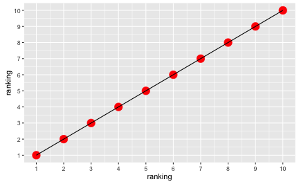
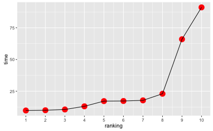
Let’s look at a practical example. Suppose 10 sprinters are running the 100 meters, with different times:

sprinters <- data.frame(
  ranking = 1:10,
  time = c(9.8, 10, 10.6, 13.1, 17.2, 17.3, 17.8, 23, 66, 91.1)
)

Of course, the rankings appear equidistant:

library(ggplot2)
ggplot(sprinters, aes(x = ranking, y = ranking)) + geom_point(color = "red", size = 5) +
  geom_line() + scale_x_continuous(breaks = 1:10) +
  scale_y_continuous(breaks = 1:10)

But the running times clearly are not:

ggplot(sprinters, aes(x = ranking, y = time)) + geom_point(color = "red", size = 5) +
  geom_line() +
  scale_x_continuous(breaks = 1:10)

Enough values = metric level?

Some say (sorry, did not find a citation, but one of my teachers said so!) that if there are “enough” values, the variable becomes “automagically” metric. I cannot see why this must necessarily happen. Suppose we would not have 10 but 100 sprinters; the picture and the argument would in essence remain the same. Equidistance will not necessarily pop out. It may by chance occur, but it is not a necessity (by far not).

Now, if we were to have many items, can we then infer that equidistance will necessarily come out? Let’s put it this way in our sprinter example: Suppose we had not watched one race, but many (say, 8). Assume that the measurement error is negligible (to make things easier but without loss of generality). If measurement error is negligible, then the actual performance, ie., the sprint times, can be taken to be the “real” (“latent”) sprinting time of the person. Measurement error is not only confined to e.g., imprecision when taking the time, but includes local particularities as wind speed, mood disturbances, bad hair days, etc.

Then, again, I think, the argument remains the same: We would have more data, but in this toy example, the average time values of the sprinters would remain the same as in the example above. So the implications also remain the same. Equidistance is no free lunch.

If ordinal and metric association measures are similar, then what the fuss?

Some argue in this way: Association measures (such as Kendall’s tau) and metric association measures (such as Pearson’ r) are often similar.

Hence, it is inferred that it does not matter much if we take the ranks as metric variables. I disagree with that argument.

What follows is inspired by Gigerenzer’s 1981 book (available in German only). Let’s first come up with some data (taken from Gigerenzer’s book, p. 303):

df <- data.frame(
  x = c(-2, -2, -1, 0, 0, 1, 1, 3, 5, 5),
  y = c(0, 0.5, 1, 1.5, 2, 13, 13.5, 14, 14.5, 15),
  ID = 1:10
)

This yields a correlation (Pearson) of

r_pearson <- round(cor(df$x, df$y), 3)
r_pearson
## [1] 0.868

a Spearman correlation of

r_spearman <- round(cor(df$x, df$y, method = "spearman"), 3)
r_spearman
## [1] 0.988

and Kendall’s tau of

tau <- round(cor(df$x, df$y, method = "kendall"), 3)
tau
## [1] 0.955

r squared is 0.753424.

Ordinal association is perfect if the ranking in both variables is identical. Let’s visualize ordinal association. Visually, as in the following diagram, this amounts to non-intersecting lines:

library(tidyr)

df_long <- tidyr::gather(df, key = variable, value = value, -ID)
# df_long

ggplot(df_long, aes(x = variable, y = value)) + geom_point() +
  geom_line(aes(group = ID))

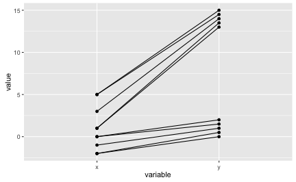
As can be seen in the diagram above, the lines are not intersecting. So the ordinal association measures should be (close to) 1. Actually, we have some ties, that’s why our measures (Spearman, Kendall) are not perfectly one. Note that the raw value are depicted.

Now let’s visualize Pearson correlation. Pearson’s r can be seen as a function of the z-values, so let’s depict z-values of a perfect correlation as a first step.

df_z <- data.frame(scale(df))
df_z$ID <- 1:10
df_z$y <- df_z$x

df_z_long <- gather(df_z, key = variable, value = value, -ID)
ggplot(df_z_long, aes(x = variable, y = value)) + geom_point() +
  geom_line(aes(group = ID))

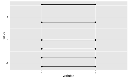
Perfect correlations amounts to horizontal lines in our diagram (remember that z-values are used instead of raw values.) Now let’s look at our example data in the next step.

df_z <- data.frame(scale(df))
df_z$ID <- 1:10
df_z_long <- gather(df_z, key = variable, value = value, -ID)


# df_z_long
ggplot(df_z_long, aes(x = variable, y = value)) + geom_point() +
  geom_line(aes(group = ID))

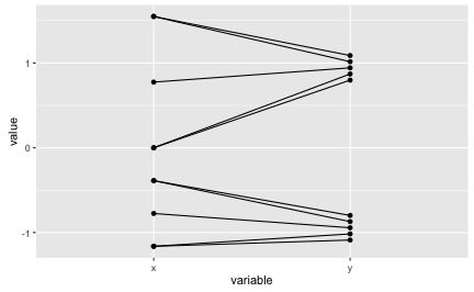
The lines are far from being horizontal. The z-values are quite different between the two variables as can be seen in the diagram. But still, Pearson’s r is very high. We must infer that strong ordinal assocation is enough to get r really high.

We see that a high r does not guarantee that the z-values between the two variables are similar. Similarly, if both the ordinal association measure (Spearman, Kendall) and the metric association measure (Pearson r) are high, we cannot infer that the metric values and the ranks are identical or very similar.

That’s why I emphatically insist that e.g., Labovitz 1970 is outright wrong when he argues that r and rho yields similar numbers, hence, ordinal can be taken as metric.

It may seem bewildering that the standard deviation (sd) of a vector X is (generally) unequal to the mean absolute deviation from the mean (MAD) of X, ie.

\(sd(X) \ne MAD(X)\).

One could now argue this way: well, sd(X) involves computing the mean of the squared \(x_i\), then taking the square root of this mean, thereby “coming back” to the initial size or dimension of x (i.e, first squaring, then taking the square root). And, MAD(X) is nothing else then the mean deviation from the mean. So both quantities are very similar, right? So one could expect that both statistics yield the same number, given they operate on the same input vector X.

However, this reasoning if flawed. As a matter of fact, sd(X) will almost certainly differ from MAD(X).

This post tries to give some intuitive understanding to this matter.

Well, we could of course lay back and state that why for heaven’s sake should the two formulas (sd and MAD) yield the same number? Different computations are involved, so different numbers should pop out. This would cast the burden of proof to the opposite party (showing that there are no differences). However, this answer does not really appeal if one tries to understand why it things are the way they are. So let’s try to develop some sense out of it.

Looking at the formulas

The formula above can be written out as

\[\sqrt{\frac{1}{n} \sum{x^2_i}} \ne \frac{1}{n} \sum{x_i}\]

where \(X\) is a vector of some numeric values. For the sake of simplicity \(x_i\) refers to the difference of some value to its mean.

Looking at the formula above, our question may be more poignantly formulated as “why does the left hand side where we first square and then take the opposite operation, square root, does not yield the same number as the right hand side?”. Or similarly, why does the square root not “neutralize” or “un-do” the squaring?

If we suspect that the squaring-square-rooting is the culprit, let’s simplify the last equation a bit, and kick-out the \(\frac{1}{n}\) part. But note that we are in fact changing the equation here.

For generality, let’s drop the notion that \(x_i\) necessarily stands for the difference of some value of a vector to the mean of the vector. We just say now that \(x_i\) is some numeric value whatsoever (but positive and real, to make life easier).

Then we have:

\[\sqrt{ \sum{x^2_i}} \ne \sum{x_i}\]

This equation is much nicer in the sense it shows the problem clearer. It is instructive to now square both sides:

\[\sum{x^2_i} \ne (\sum{x_i})^2\]

In words, our problem is now “Why is the sum of squares different to the square of the sum?”. This problem may sound familiar and can be found in a number of application (eg., some transformation of the variance).

Let’s further simplify (but without breaking rules at this point), and limit our reasoning to a vector X of two values only, a and b:

\[a^2 + b^2 \ne (a+b)^2\]

Oh, even more familiar. We clearly see a binomial expression here. And clearly:

\[a^2 + b^2 \ne (a+b)^2 = a^2 + 2ab + b^2\]

Visualization

A helpful visualization is this:

visulization of binomial theorem.

This scheme makes clear that the difference between the left hand side and the right hand side are the two green marked areas. Both are \(ab\), so \(2ab\) in total. \(2ab\) is the difference between the two sides of the equation.

Going back to the average (1/n)

Remember that above, we deliberately changed the initial equation (the initial problem). That is, we changed the equation in a non-admissible way in order to render the problem more comprehensible and more focused. Some may argue that we should come back to the initial problem, where not sums but averages are to be computed. This yields a similar, but slightly more complicated reasoning.

Let us again stick to a vector X with two values (a and b) only. Then, the initial equation becomes:

\[\sqrt{ \frac{a^2}{2} + \frac{b^2}{2}} \ne \frac{a}{2} + \frac{b}{2}\]

Squaring both sides yields

\[\frac{a^2}{2} + \frac{b^2}{2} \ne (\frac{a}{2} + \frac{b}{2})^2\]

This can be simplified (factorized) as

\(\frac{1}{2} (a^2 + b^2) \ne \frac{1}{2^2}(a^2 + 2ab + b^2)\).

Now we have again a similar situation as above. The difference being that on the left hand side (1/2) if factored out; on the right hand side (1/4) is factored out. As the formulas are different (and similar to our reasoning above), we could stop and argue that is unlikely that both sides yield the same value.

Visualization 2

As a final step, let’s visualize the thoughts of the previous lines.

What this amazing forest of crossing lines wants to tell you is the following. For the left hand side, the diagonal lines divide \(a^2\) and \(b^2\) in two parts of equal size, i.e., \(a^2/2\) and \(b^2/2\).

For the right hand side, a similar idea applies. But the double-crossed (“x-type”) lines indicate that each of the four forms is divided in 4 equal parts, ie., \(a^2/4\), \(b^2/4\) and two times \(ab/4\).

From this sketch, again it appears unlikely that both sides would yield the same number. We have not proven that is impossible, but our reasoning suggests that it would be highly unlikely to see the same number on both sides of the equation.