Markdown is thought as a “lightweight” markup language, hence the name markdown. That’s why formatting options are scarce. However, there are some extensions, for instance brought by RMarkdown.

One point of particular interest is the sizing of figures. Let’s look at some ways how to size a figure with RMarkdown.

We take some data first:

data(mtcars) 
names(mtcars) 

##  [1] "mpg"  "cyl"  "disp" "hp"   "drat" "wt"   "qsec" "vs"   "am"   "gear"
## [11] "carb"

Not let’s plot.

Define size in YAML header

We can define the size of figures globally in the YAML part, like this for example.

--- 
title: "My Document" 
output: html_document: 
fig_width: 6 
fig_height: 4 
--- 

Defining figures size for R plots

Define figure size as global chunk option

As a first R-chunk in your RMD document, define the general chunk settings like this:

knitr::opts_chunk$set(fig.width=12, fig.height=8) 

Chunk options

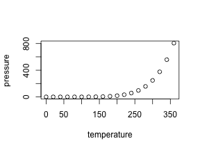
We can set the chunk options for each chunk too. With figh.height and fig.width we can define the size. Note that the numbers default to inches as unit: {r fig1, fig.height = 3, fig.width = 5}.

plot(pressure) 

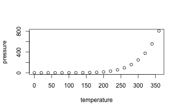
For a plot of different size, change simple the numbers: {r fig2, fig.height = 3, fig.width = 3, fig.align = "center"}.

plot(pressure) 

Alternatively, you may change the aspect ratio of the image: {r fig3, fig.width = 5, fig.asp = .62}.

plot(pressure) 

Note that the aspect ratio is based on the fig.width specified by you. See here.

Different options for different output formats

The options for figure sizing also depend on the output format (HTML vs. Latex, we do not mention Word here). For instance, in Latex percentage is allowed, as is specified on the options page: {r fig4, out.width = '40%'}.

plot(pressure) 

But note that it appears to work in HTML too.

Differnce between figure size and output size

We are allowed to specify the figure size, and secondly the size of the figure as to appear in the output. For example, if you set the size of a ggplot figure to large, then fonts etc. will appear tiny. Better do not scale up fig.height, but set out.width accordingly, eg., like this out.width = "70%".

Using Pandoc’s Markdown for figure sizing

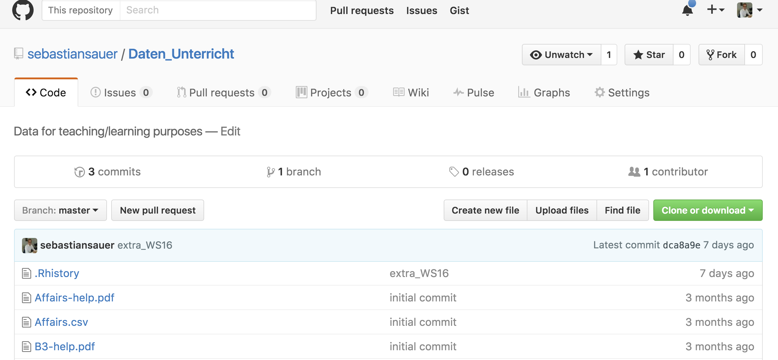
Alternatively, instead of using R for plotting, you can just load an image. Of course, it is possible to just use markdown for that: ![](path/to/figure/figure.png).

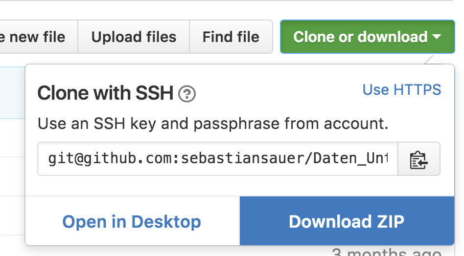
Change the figure size like this: ![](file.jpg){ width=50% }. Note that no space are allowed around the = (equal sign), and the curly brace { needs to come right after the ) brace; no space allowed.

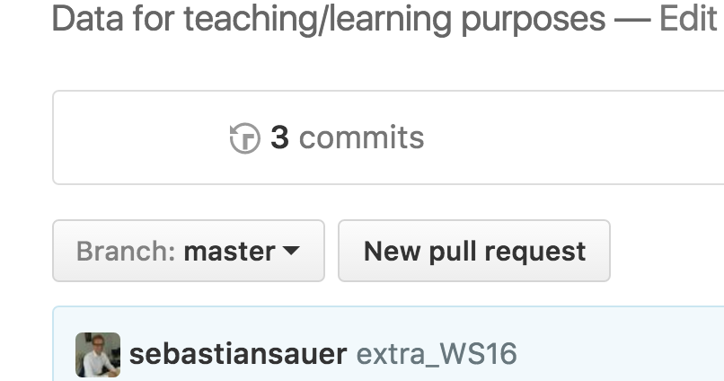
Similarly, with path to local folder:

![](../../sebastiansauer.github.io/images/2016-10-17/unnamed-chunk-5-1.png.png)

{ width=20% }

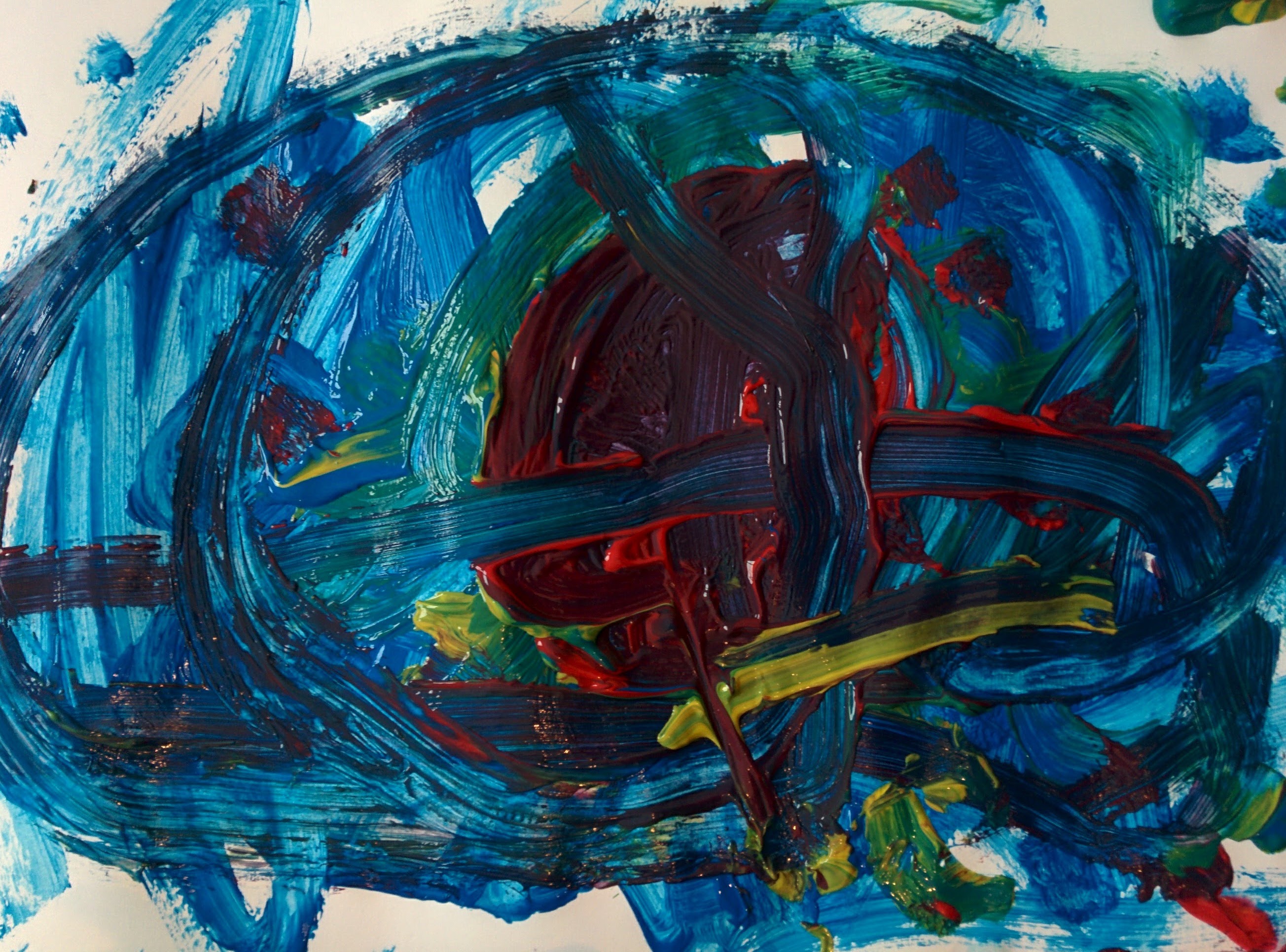
Centering is not really part of markdown. But there are some workarounds. See:

I used this code:

<center>
![](https://sebastiansauer.github.io/images/2016-10-17/unnamed-chunk-5-1.png){
width=20% }
</center>

Using the knitr function include_graphics

We can use the knitr function include_graphics which is convenient, as it takes care for the different output formats and provides some more features (see here the help file).

Note that online sources are allowed. Don`t forget to load knitr previously.

If all fails

Just resize the image with your favorite photo/image manager such as Gimp, Photoshop, Preview App etc.

Further reading Finde good advice on Yihui’s option page

here. The Book “R for Data Science” by Hadley Wickham and Garrett Grolemund (read here) is a great resource too. Read chapter 28 on diagrams here. Pandoc’s user guide has some helpful comments on figures sizing with Pandoc’s markdown .

In data analysis, we often ask “Do these two groups differ in the outcome variable”? Asking this question, a tacit assumption may be that the grouping variable is the cause of the difference in the outcome variable. For example, assume the two groups are “treatment group” and “control group”, and the outcome variable is “pain reduction”.

A typical approach would be to report the strenght of the difference by help of Cohen’s d. Even better (probably, but this atttitude is not undebated) is to report confidence intervals for d.

Although this approach is widely used, I think it is not ideal. One reason is that we (may) have tacitly changed our hypothesis. We are not asking anymore “Do individuals between the two groups differ?” but we ask now “Do the mean values differ?”, which is different. Although we are used to this approach, there are problems: Often, our theories do not state that e.g., some pill will change the mean of a group. Rather, the theory will (quite rightly, in principle) suggest that some chemical compound in an organism will change some molecules, thereby some cell metabolism products, and finally bringing about some biological and/or psychological change (to the better). This is complete different a theory. And the last theory makes sense (potentially) from a biological and logical perspective. The former does not make any sense. How can some chemical affect some group averages, some “average organism” which does not exist in reality? If we agre with that notion we would be forced, I believe, not to compare means.

But what can we do instead? In fact, some new methods have been proposed; for example James Grice developed what he has dubbed Observation Oriented Moeling. But maybe an easy, first step alternative could be using the “common language effect size” (CLES). CLES simply states “given the observed effect, how likely is it that if we draw two individuals, one from each of the two groups, that the individual from the experimental group will have a higher value in the variable of interest?” (see here).

The value of CLEs is observational, not a hypothetical parameter. It is quite straight-forward man-on-the-street logic. For example: “Draw 100 pairs from the two groups; in 83 cases the experimental group person will a higher value”. That makes sense from an observation or individual organism point of view.

Practically, there are R packages out there which help us computing CLES (or at least one package). The details of the computation are beyond the scope of this article; see here for mathematical details.

Rather, we will build a nice plot for displaying a number of CLES differences between two groups.

First, let’s get some data, and load the needed packages.

library(tidyverse)

# library(readr)
extra_file <- "https://raw.github.com/sebastiansauer/Daten_Unterricht/master/extra.csv"

extra_df <- read_csv(extra_file)

This dataset extra comprises answers to a survey tapping into extraversion as a psychometric variable plus some related behavior (e.g., binge drinking). The real-word details are not so much of interest here.

So, let’s pick all numeric variables plus one grouping variable (say, sex):

# library(dplyr)
extra_df %>% 
  na.omit() %>% 
  select_if(is.numeric) %>% 
  names -> extra_num_vars

First, we compute a t-test for each numeric variable (using our grouping variable “sex”):

# library(purrr)
extra_df %>% 
  dplyr::select(one_of(extra_num_vars)) %>% 
  # na.omit() %>% 
  map(~t.test(. ~ extra_df$Geschlecht)) %>% 
  map(~compute.es::tes(.$statistic,
                       n.1 = nrow(dplyr::filter(extra_df, Geschlecht == "Frau")),
                       n.2 = nrow(dplyr::filter(extra_df, Geschlecht == "Mann")))) %>% 
  map(~do.call(rbind, .)) %>% 
  as.data.frame %>% 
  t %>% 
  data.frame %>% 
  rownames_to_column %>% 
  rename(outcomes = rowname) -> 
  extra_effsize

Note: output hidden, tl;dr.

Puh, that’s a bit confusing. So, what did we do?

1. We selected the numeric variables of the data frame; here one_of comes handy. This function gets the column names of a data frame as input, and allows to select all of them in the select function.
2. We mapped a t-test to each of those columns, where extra_df$Geschlecht was the grouping variable. Note that the dot . is used as a shortcut for the lefthand side of the equation, ie., whatever is handed over by the pipe ` %>% ` in the previous line/step.
3. Next, we computed the effect size using tes from package compute.es.
4. For each variable submitted to a t-test, bind the results rowwise. Each t-test gives back a list of results. We want to bind those results in a list. As we have several list elements (for each t-test), we can use do.call to bind that all together in one go.
5. Convert to data frame.
6. Better turn matrix by 90° using t.
7. As t gives back a matrix, we need to convert to data frame again.
8. Rownames should be their own column with an appropriate name (outcomes).
9. Save that in an own data frame.

And compute the differences in CLES, and plot it:

# library(ggplot2)
extra_effsize %>% 
  dplyr::select(outcomes, cl.d) %>% 
  mutate(sign = ifelse(cl.d > 50, "+", "-")) %>% 
  ggplot(aes(x = reorder(outcomes, cl.d), y = cl.d, color = sign)) + 
  geom_hline(yintercept = 50, alpha = .4) +
  geom_point(aes(shape = sign)) + 
  coord_flip() +
  ylab("effect size (Common Language Effect Size)") +
  xlab("outcome variables") + 
  ggtitle("CLES plot") -> CLES_plot


CLES_plot

The code above in more detail:

1. select columns outcomes and cl.d; note that cl.d stands for CLES (here: Common Language Cohen’s d, as CLES is derived from Cohen’s d).
2. Compute variable to tell in which direction the difference points, ie., whether it is greater or smaller than 50%, where 50% refers to ignorance towards the direction of difference.
3. Well, now plot, but sort the outcomes by their CLES value; for the purpose of sorting we use reorder.
4. Flip the axes because it is more beautiful here.

Often, we want to check for missing values (NAs). There are of course many ways to do so. dplyr provides a quite nice one.

First, let’s load some data:

library(readr)
extra_file <- "https://raw.github.com/sebastiansauer/Daten_Unterricht/master/extra.csv"

extra_df <- read_csv(extra_file)

Note that extra is a data frame consisting of survey items regarding extraversion and related behavior.

In case the dataframe is quite largish (many columns) it is helpful to have some quick way. Here, we have 25 columns. That is not enormous, but ok, let’s stick with that for now.

library(dplyr)

extra_df %>% 
  select_if(function(x) any(is.na(x))) %>% 
  summarise_each(funs(sum(is.na(.)))) -> extra_NA

So, what have we done? The select_if part choses any column where is.na is true (TRUE). Then we take those columns and for each of them, we sum up (summarise_each) the number of NAs. Note that each column is summarized to a single value, that’s why we use summarise. And finally, the resulting data frame (dplyr always aims at giving back a data frame) is stored in a new variable for further processing.

Now, let’s see:

# library(pander)  # for printing tables in markdown
library(knitr)

kable(extra_NA)

Subsetting a data frame is an essential and frequently performed task. Here, some basic ideas are presented.

Get some data first.

str(mtcars)

## 'data.frame':	32 obs. of  11 variables:
##  $ mpg : num  21 21 22.8 21.4 18.7 18.1 14.3 24.4 22.8 19.2 ...
##  $ cyl : num  6 6 4 6 8 6 8 4 4 6 ...
##  $ disp: num  160 160 108 258 360 ...
##  $ hp  : num  110 110 93 110 175 105 245 62 95 123 ...
##  $ drat: num  3.9 3.9 3.85 3.08 3.15 2.76 3.21 3.69 3.92 3.92 ...
##  $ wt  : num  2.62 2.88 2.32 3.21 3.44 ...
##  $ qsec: num  16.5 17 18.6 19.4 17 ...
##  $ vs  : num  0 0 1 1 0 1 0 1 1 1 ...
##  $ am  : num  1 1 1 0 0 0 0 0 0 0 ...
##  $ gear: num  4 4 4 3 3 3 3 4 4 4 ...
##  $ carb: num  4 4 1 1 2 1 4 2 2 4 ...

mtcars <- head(mtcars)  # for shorter output
mtcars

##                    mpg cyl disp  hp drat    wt  qsec vs am gear carb
## Mazda RX4         21.0   6  160 110 3.90 2.620 16.46  0  1    4    4
## Mazda RX4 Wag     21.0   6  160 110 3.90 2.875 17.02  0  1    4    4
## Datsun 710        22.8   4  108  93 3.85 2.320 18.61  1  1    4    1
## Hornet 4 Drive    21.4   6  258 110 3.08 3.215 19.44  1  0    3    1
## Hornet Sportabout 18.7   8  360 175 3.15 3.440 17.02  0  0    3    2
## Valiant           18.1   6  225 105 2.76 3.460 20.22  1  0    3    1

One: Addressing dataframe as list (vector, 1-dim structure)

Data frames can be understood/addressed as lists, ie., as some type of vectors. Vectors have one dimension. Thus, we can access/subset with one index only (one dimension). For example mtcars[1] selects the first element (ie., column) of mtcars.

mtcars[1]

##                    mpg
## Mazda RX4         21.0
## Mazda RX4 Wag     21.0
## Datsun 710        22.8
## Hornet 4 Drive    21.4
## Hornet Sportabout 18.7
## Valiant           18.1

mtcars["mpg"]

##                    mpg
## Mazda RX4         21.0
## Mazda RX4 Wag     21.0
## Datsun 710        22.8
## Hornet 4 Drive    21.4
## Hornet Sportabout 18.7
## Valiant           18.1

mtcars[c("mpg", "cyl")]  

##                    mpg cyl
## Mazda RX4         21.0   6
## Mazda RX4 Wag     21.0   6
## Datsun 710        22.8   4
## Hornet 4 Drive    21.4   6
## Hornet Sportabout 18.7   8
## Valiant           18.1   6

mtcars[1:3]

##                    mpg cyl disp
## Mazda RX4         21.0   6  160
## Mazda RX4 Wag     21.0   6  160
## Datsun 710        22.8   4  108
## Hornet 4 Drive    21.4   6  258
## Hornet Sportabout 18.7   8  360
## Valiant           18.1   6  225

Note that data frames are vectors (lists) technically, where the vectors are the columns and the columns possess names. Thus we can address the columns by their names. Of course, we can select (address/index/subset) more than one element (column) using the c() function.

Besides names, we can address the elements by their number: type a positive integer to subset the respective element. c can be used here too.

Note that the : (colon) operator is a short hand for c(from_this_column_to_that column).

Similarly to addressing the names of the data frames using brackets [], we can use the Dollar $ operator:

mtcars$mpg

## [1] 21.0 21.0 22.8 21.4 18.7 18.1

Whatever comes after the $ is understood by R as the name (without quotation marks) of the column within that data frame. $ is a shorthand for [[]] (but not exactly the same; see here for an excellent overview).

Two: Addressing dataframe as a matrix (2-dim-structure, 2-dim-matrix)

As data frames can also be addressed as rectangular, two-dimensional matrices, we may subset specific elements using a x-y-coordinate scheme where in R matrices the row is addressed first, and the column second, eg., mtcars(1,2) would be first line of second column.

mtcars[1,1]

## [1] 21

mtcars[1, c(1,2)]

##           mpg cyl
## Mazda RX4  21   6

mtcars[1, 1:3]

##           mpg cyl disp
## Mazda RX4  21   6  160

mtcars[1, c(1:3)]

##           mpg cyl disp
## Mazda RX4  21   6  160

mtcars[, c(1:3)]

##                    mpg cyl disp
## Mazda RX4         21.0   6  160
## Mazda RX4 Wag     21.0   6  160
## Datsun 710        22.8   4  108
## Hornet 4 Drive    21.4   6  258
## Hornet Sportabout 18.7   8  360
## Valiant           18.1   6  225

mtcars[1, "mpg"]

## [1] 21

mtcars[1, c("mpg", "cyl")]  

##           mpg cyl
## Mazda RX4  21   6

Again, the c() operator may be used to group several rows or columns. Columns may again addressed by their names (row names are unusual). The : colon operator is allowed, too.

Three: Logical subsetting in dataframes

mtcars[c(T, T, F, F, F, F, F, F, F, F, T)]

##                    mpg cyl carb
## Mazda RX4         21.0   6    4
## Mazda RX4 Wag     21.0   6    4
## Datsun 710        22.8   4    1
## Hornet 4 Drive    21.4   6    1
## Hornet Sportabout 18.7   8    2
## Valiant           18.1   6    1

mtcars[c(T, T, F)]

##                    mpg cyl  hp drat  qsec vs gear carb
## Mazda RX4         21.0   6 110 3.90 16.46  0    4    4
## Mazda RX4 Wag     21.0   6 110 3.90 17.02  0    4    4
## Datsun 710        22.8   4  93 3.85 18.61  1    4    1
## Hornet 4 Drive    21.4   6 110 3.08 19.44  1    3    1
## Hornet Sportabout 18.7   8 175 3.15 17.02  0    3    2
## Valiant           18.1   6 105 2.76 20.22  1    3    1

In the first example above, the columns #1, #2, #and #11 are selected, because their position is indexed as TRUE (or T).

Note that if you supply less elements than the length of the objects (eg., here 11 columns/elements), R will recycle your elements until the full length of the element is met (here: TTF-TTF-TTF-TT).

Again, the data frame can be addressed either as a list (1-dim), or as a 2-dim matrix. See here for an example using logical indexing and addressing the data frame as a 2-dim matrix:

mtcars[c(T, T, F), c(T, T, F)]

##                    mpg cyl  hp drat  qsec vs gear carb
## Mazda RX4         21.0   6 110 3.90 16.46  0    4    4
## Mazda RX4 Wag     21.0   6 110 3.90 17.02  0    4    4
## Hornet 4 Drive    21.4   6 110 3.08 19.44  1    3    1
## Hornet Sportabout 18.7   8 175 3.15 17.02  0    3    2

Actually, the logical subsetting is quite powerful. We can use a predicate function, ie., a function delivering a logial state (TRUE or FALSE) within the subsetting:

mtcars[mtcars$cyl == 6, c(1,2)]

##                 mpg cyl
## Mazda RX4      21.0   6
## Mazda RX4 Wag  21.0   6
## Hornet 4 Drive 21.4   6
## Valiant        18.1   6

Here, we declared that we only want rows for which the following condition is TRUE: mtcars$cyl == 6. (And only cols 1 and 2.)

Final words

Subsetting in R is an essential task. It is also not so easy, as many slightly different variants exist. Here, only some ideas were presented. A much broader are excellently presented by Hadley Wickham here.

Besides that subsettting using base R should be well understood, it may be more comfortable to use functions such as select from dplyr.

Downloading a folder (repository) from Github as a whole

The most direct way to get data from Github to your computer/ into R, is to download the repository. That is, click the big green button:

The big, green button saying “Clone or download”, click it and choose “download zip”.

Of course, for those using Git and Github, it would be appropriate to clone the repository. And, although appearing more advanced, cloning has the definitive advantage that you’ll enjoy the whole of the Github features. In fact, the whole purpose of Github is to provide a history of the file(s), so the purpose is not really served if one just downloads the most recent snapshot. But anyhow, that depends on you own will.

Note that “repository” can be thought of as “folder” or “project”.

Once downloaded, you need to unzip the folder. Unzipping means to “extract” or “unpack” the file/folder. On many machines, this can be accomplished by right clicking the icon and choosing something like “extract here”.

Once extracted, just navigate to the folder and open whatever file you are inclined to.

Downloading individual files from Github

In case you do not want to download the whole repository, individual files can be downloaded and parsed to R quite easily:

library(readr)  # for read_csv
library(knitr)  # for kable
myfile <- "https://raw.github.com/sebastiansauer/Daten_Unterricht/master/Affairs.csv"

Affairs <- read_csv(myfile)

## Warning: Missing column names filled in: 'X1' [1]

## Parsed with column specification:
## cols(
##   X1 = col_integer(),
##   affairs = col_integer(),
##   gender = col_character(),
##   age = col_double(),
##   yearsmarried = col_double(),
##   children = col_character(),
##   religiousness = col_integer(),
##   education = col_integer(),
##   occupation = col_integer(),
##   rating = col_integer()
## )

kable(head(Affairs))

Let’s quickly deconstruct the url above from Github. In general, we need to write:

https://raw.github.com/user/repository/branch/file.name.

In many cases, the branch will be “master”. You can easily find out about that one the page of the repo you wanna download:

I’ve noticed that unzipping a repository from Github (and downloading a zip file) can cause confusion, so it might be easier to provide a code bit as shown above.

BTW: read.csv should work equally.