A handy function to iterate stuff is the function purrr::map. It takes a function and applies it to all elements of a given vector. This vector can be a data frame - which is a list, tecnically - or some other sort of of list (normal atomic vectors are fine, too).

However, purrr::map is designed to return lists (not dataframes). For example, if you apply mosaic::favstats to map, you will get some favorite statistics for some variable:

library(mosaic)
library(tidyverse)

data(tips, package = "reshape2")
favstats(tips$tip)

##  min Q1 median     Q3 max     mean       sd   n missing
##    1  2    2.9 3.5625  10 2.998279 1.383638 244       0

Note that favstats does not accept several columns/variables as parameters; one only at a time is permitted.

Ok, let’s apply favstats to each numeric column of our dataframe:

tips %>% 
  select_if(is.numeric) %>% 
  map(mosaic::favstats)

## $total_bill
##   min      Q1 median      Q3   max     mean       sd   n missing
##  3.07 13.3475 17.795 24.1275 50.81 19.78594 8.902412 244       0
## 
## $tip
##  min Q1 median     Q3 max     mean       sd   n missing
##    1  2    2.9 3.5625  10 2.998279 1.383638 244       0
## 
## $size
##  min Q1 median Q3 max     mean        sd   n missing
##    1  2      2  3   6 2.569672 0.9510998 244       0

Quite nice, but we are given back a list with several elements; each element is a “row” of our to-be dataframe. How to change this list to a regular dataframe (tibble)?

This trick can be solved by use of some sort of repeated rbind. rbind binds rows together, hence the name. But rbinds does only accept two elements as input. Now comes do.call to help. Effectiveley, do.call does something like: rbind(my_list[[1]], my_list[[2]], my_list[[2]], ...) (this is pseudo code).

tips %>% 
  select_if(is.numeric) %>% 
  map(mosaic::favstats) %>% 
  do.call(rbind, .)

##             min      Q1 median      Q3   max      mean        sd   n
## total_bill 3.07 13.3475 17.795 24.1275 50.81 19.785943 8.9024120 244
## tip        1.00  2.0000  2.900  3.5625 10.00  2.998279 1.3836382 244
## size       1.00  2.0000  2.000  3.0000  6.00  2.569672 0.9510998 244
##            missing
## total_bill       0
## tip              0
## size             0

Note the little dot in rbind.

Now be happy with the dataframe :-)

One nice features of .rmd files is that version control systems, such as git and github, can (quite) easily be combined. However, in my experience, merge conflicts are not so uncommon. That raises the question how to avoid merge conflicts when syncing with Github?

Here’s a quick overview on what to do to that hassle:

1. Sync often.
2. Hard wrap the lines to approx. 80 characters.
3. Pull before you start to change the source files.

Watch out not to hard wrap YAML. Some Latex code also does not like being hard wrapped (some functions need their own, new line to be executed properly).

Hier eine Liste einiger meiner “Lieblings-R-Funktionen”; für Einführungsveranstaltungen in Statistik spielen sie (bei mir) eine wichtige Rolle. Die Liste kann sich ändern :-)

Wenn ich von einer “Tabelle” spreche, meine ich sowohl Dataframes als auch Tibbles.

Zuweisung - <-

Mit dem Zuweisungsoperator <- kann man Objekten einen Wert zuweisen:

x <- 1
mtcars2 <- mtcars

Spalten als Vektor auswählen - $

Mit dem Operator $ kann man eine Spalte einer Tabelle auswählen. Die Spalte wird als Vektor zurückgegeben.

mtcars$hp

##  [1] 110 110  93 110 175 105 245  62  95 123 123 180 180 180 205 215 230
## [18]  66  52  65  97 150 150 245 175  66  91 113 264 175 335 109

Struktur eines Objekts ausgeben lassen - str

Die “Struktur” eines Objekts (z.B. einer Tabelle) kann man sich mit str ausgeben lassen:

str(mtcars)

## 'data.frame':	32 obs. of  11 variables:
##  $ mpg : num  21 21 22.8 21.4 18.7 18.1 14.3 24.4 22.8 19.2 ...
##  $ cyl : num  6 6 4 6 8 6 8 4 4 6 ...
##  $ disp: num  160 160 108 258 360 ...
##  $ hp  : num  110 110 93 110 175 105 245 62 95 123 ...
##  $ drat: num  3.9 3.9 3.85 3.08 3.15 2.76 3.21 3.69 3.92 3.92 ...
##  $ wt  : num  2.62 2.88 2.32 3.21 3.44 ...
##  $ qsec: num  16.5 17 18.6 19.4 17 ...
##  $ vs  : num  0 0 1 1 0 1 0 1 1 1 ...
##  $ am  : num  1 1 1 0 0 0 0 0 0 0 ...
##  $ gear: num  4 4 4 3 3 3 3 4 4 4 ...
##  $ carb: num  4 4 1 1 2 1 4 2 2 4 ...

Die Tabelle mtcars ist ein data.frame mit 32 Fällen und 11 Variablen. Alle Variablen sind numerisch (num).

Werte zu einem Vektor zusammenfügen - c

Einzelne Werte kann man man c (wie “combine”) zu einem Vektor zusammenfügen.

x <- c(1,2,3)
x

## [1] 1 2 3

y <- c(1)

z <- c("Anna", "Berta", "Carla")

Zu beachten ist, dass ein Vektor nur einen Typ von Daten (z.B. nur Text oder nur reelle Zahlen) enthalten kann. Im Zweifel macht R aus dem Vektor einen Text-Vektor.

Nur die ersten Zeilen einer Tabelle anzeigen - head

Mit head kann man sich die ersten Zeilen einer Tabelle anzeigen lassen:

head(mtcars)  # 6 Zeilen sind der Default-Wert

##                    mpg cyl disp  hp drat    wt  qsec vs am gear carb
## Mazda RX4         21.0   6  160 110 3.90 2.620 16.46  0  1    4    4
## Mazda RX4 Wag     21.0   6  160 110 3.90 2.875 17.02  0  1    4    4
## Datsun 710        22.8   4  108  93 3.85 2.320 18.61  1  1    4    1
## Hornet 4 Drive    21.4   6  258 110 3.08 3.215 19.44  1  0    3    1
## Hornet Sportabout 18.7   8  360 175 3.15 3.440 17.02  0  0    3    2
## Valiant           18.1   6  225 105 2.76 3.460 20.22  1  0    3    1

head(mtcars, 3)  # nur die ersten 3 Zeilen etc.

##                mpg cyl disp  hp drat    wt  qsec vs am gear carb
## Mazda RX4     21.0   6  160 110 3.90 2.620 16.46  0  1    4    4
## Mazda RX4 Wag 21.0   6  160 110 3.90 2.875 17.02  0  1    4    4
## Datsun 710    22.8   4  108  93 3.85 2.320 18.61  1  1    4    1

Spalten auswählen - dplyr::select

Spalten kann man mit select auswählen:

library(tidyverse) # oder: library(dplyr)
select(mtcars, hp, cyl)

##                      hp cyl
## Mazda RX4           110   6
## Mazda RX4 Wag       110   6
## Datsun 710           93   4
## Hornet 4 Drive      110   6
## Hornet Sportabout   175   8
## Valiant             105   6
## Duster 360          245   8
## Merc 240D            62   4
## Merc 230             95   4
## Merc 280            123   6
## Merc 280C           123   6
## Merc 450SE          180   8
## Merc 450SL          180   8
## Merc 450SLC         180   8
## Cadillac Fleetwood  205   8
## Lincoln Continental 215   8
## Chrysler Imperial   230   8
## Fiat 128             66   4
## Honda Civic          52   4
## Toyota Corolla       65   4
## Toyota Corona        97   4
## Dodge Challenger    150   8
## AMC Javelin         150   8
## Camaro Z28          245   8
## Pontiac Firebird    175   8
## Fiat X1-9            66   4
## Porsche 914-2        91   4
## Lotus Europa        113   4
## Ford Pantera L      264   8
## Ferrari Dino        175   6
## Maserati Bora       335   8
## Volvo 142E          109   4

Zeilen filtern - dplyr::filter

Zeilen filtern kann man mit filter:

filter(mtcars, hp > 200, cyl > 6)

##    mpg cyl disp  hp drat    wt  qsec vs am gear carb
## 1 14.3   8  360 245 3.21 3.570 15.84  0  0    3    4
## 2 10.4   8  472 205 2.93 5.250 17.98  0  0    3    4
## 3 10.4   8  460 215 3.00 5.424 17.82  0  0    3    4
## 4 14.7   8  440 230 3.23 5.345 17.42  0  0    3    4
## 5 13.3   8  350 245 3.73 3.840 15.41  0  0    3    4
## 6 15.8   8  351 264 4.22 3.170 14.50  0  1    5    4
## 7 15.0   8  301 335 3.54 3.570 14.60  0  1    5    8

Zeilen sortieren - dplyr::arrange

Mit arrange kann man eine Tabelle nach einer Spalte filtern.

mtcars_sortiert <- arrange(mtcars, -cyl)
head(mtcars_sortiert, 3)

##    mpg cyl  disp  hp drat   wt  qsec vs am gear carb
## 1 18.7   8 360.0 175 3.15 3.44 17.02  0  0    3    2
## 2 14.3   8 360.0 245 3.21 3.57 15.84  0  0    3    4
## 3 16.4   8 275.8 180 3.07 4.07 17.40  0  0    3    3

arrange sortiert als Default aufsteigend. Möchte man absteigend sortieren, kann man ein Minuszeichen vor der zu sortierenden Variable stellen.

Befehle “durchpfeifen” - ` %>% ` (dplyr)

Befehle “verknüpfen”, d.h. hintereinander ausführen kann man mit ` %>% . Es lassen sich nicht alle Befehle verknüpfen, sondern nur Befehle, die eine Tabelle als Input und als Output vorsehen. Weil der Operator %>% ` auch “pipe” (Pfeife) genannt wird, nenne ich die Anwendung des Operators auch “durchpfeifen”. Man kann ` %>% ` auf Deutsch übersetzen mit “und dann”.

mtcars %>% 
  select(hp, cyl) %>% 
  filter(hp > 200) %>% 
  arrange(-hp)

##    hp cyl
## 1 335   8
## 2 264   8
## 3 245   8
## 4 245   8
## 5 230   8
## 6 215   8
## 7 205   8

Diese Befehlskette kann man lesen als:

Nehme die Tabelle “mtcars” UND DANN
wähle die Spalten “hp” und “cyl” UND DANN
filtere nur Zeilen mit mehr als 200 PS UND DANN
sortiere absteigend nach PS.

Das Durchpfeifen ist eine tolle Sache: spart Zeit und ist gut lesbar.

Deskriptive Statistik - mean, sum, sd, median, IQR, max, min, …

Die R-Funktionen der Statistik haben recht selbst erklärende Namen. Sie erwarten einen Vektor (Spalte) als Eingabe.

mean(mtcars$hp)

## [1] 146.6875

max(mtcars$cyl)

## [1] 8

sd(mtcars$hp)

## [1] 68.56287

Deskriptive Statistik - mosaic

Mit dem Package mosaic können eine Reihe komfortabler Funktionen für z.B. die deskriptive Statistik gerechnet werden. Besonders schön ist, dass Gruppierungen sehr einfach sind.

library(mosaic)

mean(hp ~ cyl, data = mtcars)  # entsprechend für sd, median,...

##         4         6         8 
##  82.63636 122.28571 209.21429

Funktionen aus mosaic sind häufig mit dem “Kringel” Y ~ X aufgebaut. Bei den Befehlen für deskriptive Statistik steht vor dem Kringel die Datei, die analysiert werden soll und nach dem Kringel die Gruppierungsvariable.

Praktisch ist auch die Funktion favstats, die “Favoriten-Statistiken” ausgibt:

favstats(mtcars$hp)

##  min   Q1 median  Q3 max     mean       sd  n missing
##   52 96.5    123 180 335 146.6875 68.56287 32       0

favstats(mtcars$hp ~ mtcars$cyl) 

##   mtcars$cyl min     Q1 median     Q3 max      mean       sd  n missing
## 1          4  52  65.50   91.0  96.00 113  82.63636 20.93453 11       0
## 2          6 105 110.00  110.0 123.00 175 122.28571 24.26049  7       0
## 3          8 150 176.25  192.5 241.25 335 209.21429 50.97689 14       0

Grundrechnen (Arithmetik) - +, -, *, /, …

Man kann R als Taschenrechner verwenden.

2*2

## [1] 4

1+1

## [1] 2

6 / 3

## [1] 2

6 / 4

## [1] 1.5

Zu beachten ist, dass R vektoriell rechnet.

Spalten zusammenfassen zu einer Zahl - dplyr::summarise

Der Befehl summarise (aus dplyr) fasst Spalten zu einer Zahl zusammen. Daher verkraftet er auch nur Befehle, die aus einer Spalte eine Zahl machen, z.B. mean, sd etc.

mtcars %>% 
  summarise(hp_mittelwert = mean(hp))

##   hp_mittelwert
## 1      146.6875

# oder

summarise(mtcars, hp_mittelwert = mean(hp))

##   hp_mittelwert
## 1      146.6875

Tabellen gruppieren - dplyr::group_by

Häufig möchte man Gruppen vergleichen: Parken Frauen schneller aus als Männer? Haben Autos mit 6 Zylinder im Schnitt mehr PS als solche mit 8?

mtcars %>% 
  filter(cyl > 4) %>% 
  group_by(cyl) %>% 
  summarise(hp_mittelwert = mean(hp))

## # A tibble: 2 × 2
##     cyl hp_mittelwert
##   <dbl>         <dbl>
## 1     6      122.2857
## 2     8      209.2143

Alle dplyr-Befehle verstehen die Gruppierung, die group_by in die Tabelle einfügt. Achtung: Eine mit group_by gruppierte Tabelle sieht genauso aus wie eine nicht-gruppierte Tabelle. Der Effekt macht sich nur in den folgenden Befehlen bemerkbar.

Diagramme erstellen - ggplot2::qplot

Eine flexible Art, Diagramme (“plots”) zu erstellen, ist mit qplot.

library(ggplot2)

qplot(x = cyl, y = hp, data = mtcars)

Die wichtigsten Parameter der Funktion sind X-Achse (x), Y-Achse (y) und Name der Tabelle (data).

Korrelationen (bivariat) - cor

cor(mtcars$hp, mtcars$cyl)

## [1] 0.8324475

cor(mpg ~ disp, data = mtcars)

## [1] -0.8475514

Korrelationen (Matrix) - corrr

Mit dem Paket corrr lassen sich komfortabel Korrelationsmatrizen erstellen.

library(corrr)

mtcars %>% 
  correlate 

## # A tibble: 11 × 12
##    rowname        mpg        cyl       disp         hp        drat
##      <chr>      <dbl>      <dbl>      <dbl>      <dbl>       <dbl>
## 1      mpg         NA -0.8521620 -0.8475514 -0.7761684  0.68117191
## 2      cyl -0.8521620         NA  0.9020329  0.8324475 -0.69993811
## 3     disp -0.8475514  0.9020329         NA  0.7909486 -0.71021393
## 4       hp -0.7761684  0.8324475  0.7909486         NA -0.44875912
## 5     drat  0.6811719 -0.6999381 -0.7102139 -0.4487591          NA
## 6       wt -0.8676594  0.7824958  0.8879799  0.6587479 -0.71244065
## 7     qsec  0.4186840 -0.5912421 -0.4336979 -0.7082234  0.09120476
## 8       vs  0.6640389 -0.8108118 -0.7104159 -0.7230967  0.44027846
## 9       am  0.5998324 -0.5226070 -0.5912270 -0.2432043  0.71271113
## 10    gear  0.4802848 -0.4926866 -0.5555692 -0.1257043  0.69961013
## 11    carb -0.5509251  0.5269883  0.3949769  0.7498125 -0.09078980
## # ... with 6 more variables: wt <dbl>, qsec <dbl>, vs <dbl>, am <dbl>,
## #   gear <dbl>, carb <dbl>

Möchte man das obere Dreieck “abrasieren”, da es redundant ist, so kann man das so machen:

mtcars %>% 
  correlate %>% 
  shave

## # A tibble: 11 × 12
##    rowname        mpg        cyl       disp         hp        drat
##      <chr>      <dbl>      <dbl>      <dbl>      <dbl>       <dbl>
## 1      mpg         NA         NA         NA         NA          NA
## 2      cyl -0.8521620         NA         NA         NA          NA
## 3     disp -0.8475514  0.9020329         NA         NA          NA
## 4       hp -0.7761684  0.8324475  0.7909486         NA          NA
## 5     drat  0.6811719 -0.6999381 -0.7102139 -0.4487591          NA
## 6       wt -0.8676594  0.7824958  0.8879799  0.6587479 -0.71244065
## 7     qsec  0.4186840 -0.5912421 -0.4336979 -0.7082234  0.09120476
## 8       vs  0.6640389 -0.8108118 -0.7104159 -0.7230967  0.44027846
## 9       am  0.5998324 -0.5226070 -0.5912270 -0.2432043  0.71271113
## 10    gear  0.4802848 -0.4926866 -0.5555692 -0.1257043  0.69961013
## 11    carb -0.5509251  0.5269883  0.3949769  0.7498125 -0.09078980
## # ... with 6 more variables: wt <dbl>, qsec <dbl>, vs <dbl>, am <dbl>,
## #   gear <dbl>, carb <dbl>

Die Korrelationen nach Stärke ordnen geht so:

mtcars %>% 
  correlate %>% 
  rearrange(absolute = FALSE) %>% 
  shave()

## # A tibble: 11 × 12
##    rowname        mpg         vs        drat          am       gear
##      <chr>      <dbl>      <dbl>       <dbl>       <dbl>      <dbl>
## 1      mpg         NA         NA          NA          NA         NA
## 2       vs  0.6640389         NA          NA          NA         NA
## 3     drat  0.6811719  0.4402785          NA          NA         NA
## 4       am  0.5998324  0.1683451  0.71271113          NA         NA
## 5     gear  0.4802848  0.2060233  0.69961013  0.79405876         NA
## 6     qsec  0.4186840  0.7445354  0.09120476 -0.22986086 -0.2126822
## 7     carb -0.5509251 -0.5696071 -0.09078980  0.05753435  0.2740728
## 8       hp -0.7761684 -0.7230967 -0.44875912 -0.24320426 -0.1257043
## 9       wt -0.8676594 -0.5549157 -0.71244065 -0.69249526 -0.5832870
## 10    disp -0.8475514 -0.7104159 -0.71021393 -0.59122704 -0.5555692
## 11     cyl -0.8521620 -0.8108118 -0.69993811 -0.52260705 -0.4926866
## # ... with 6 more variables: qsec <dbl>, carb <dbl>, hp <dbl>, wt <dbl>,
## #   disp <dbl>, cyl <dbl>

Und plotten so:

mtcars %>% 
  correlate %>% 
  rearrange(absolute = FALSE) %>% 
  shave() %>% 
  rplot()

Häufigkeiten zählen - count

Wie viele Brillenträger gibt es bei den Männern bzw. den Frauen in der Stichprobe? Wie häufig gibt es Autos mit 4, 6 oder 8 Zylindern? Solche Häufigkeitsauswerteungen lassen sich z.B. mit dplyr::count erledigen.

dplyr::count(mtcars,cyl)

## # A tibble: 3 × 2
##     cyl     n
##   <dbl> <int>
## 1     4    11
## 2     6     7
## 3     8    14

dplyr::count(mtcars,cyl, gear)

## Source: local data frame [8 x 3]
## Groups: cyl [?]
## 
##     cyl  gear     n
##   <dbl> <dbl> <int>
## 1     4     3     1
## 2     4     4     8
## 3     4     5     2
## 4     6     3     2
## 5     6     4     4
## 6     6     5     1
## 7     8     3    12
## 8     8     5     2

Scatterplot-Matrix - GGally::ggpairs

Eine Scatterplot-Matrix kann helfen, den Zusammenhang zwischen mehreren Variablen zu visualisieren.

data(tips, package = "reshape2")
library(GGally)

ggpairs(tips, columns = c("tip", "sex", "total_bill"), aes(fill = sex))

Regression (Lineares Modell) - lm

Um eine Regression zu berechnen, verwendet man meist den Befehl lm.

lm1 <- lm(tip ~ total_bill, data = tips)
summary(lm1)

## 
## Call:
## lm(formula = tip ~ total_bill, data = tips)
## 
## Residuals:
##     Min      1Q  Median      3Q     Max 
## -3.1982 -0.5652 -0.0974  0.4863  3.7434 
## 
## Coefficients:
##             Estimate Std. Error t value Pr(>|t|)    
## (Intercept) 0.920270   0.159735   5.761 2.53e-08 ***
## total_bill  0.105025   0.007365  14.260  < 2e-16 ***
## ---
## Signif. codes:  0 '***' 0.001 '**' 0.01 '*' 0.05 '.' 0.1 ' ' 1
## 
## Residual standard error: 1.022 on 242 degrees of freedom
## Multiple R-squared:  0.4566,	Adjusted R-squared:  0.4544 
## F-statistic: 203.4 on 1 and 242 DF,  p-value: < 2.2e-16

Man kann als Prädiktoren auch nominale Variablen verwenden:

lm2 <- lm(tip ~ sex, data = tips)
summary(lm2)

## 
## Call:
## lm(formula = tip ~ sex, data = tips)
## 
## Residuals:
##     Min      1Q  Median      3Q     Max 
## -2.0896 -1.0896 -0.0896  0.6666  6.9104 
## 
## Coefficients:
##             Estimate Std. Error t value Pr(>|t|)    
## (Intercept)   2.8334     0.1481  19.137   <2e-16 ***
## sexMale       0.2562     0.1846   1.388    0.166    
## ---
## Signif. codes:  0 '***' 0.001 '**' 0.01 '*' 0.05 '.' 0.1 ' ' 1
## 
## Residual standard error: 1.381 on 242 degrees of freedom
## Multiple R-squared:  0.007896,	Adjusted R-squared:  0.003797 
## F-statistic: 1.926 on 1 and 242 DF,  p-value: 0.1665

In diesem Fall gleicht die Regression einem t-Test.

Für diesen Post benötigte R-Pakete:

library(stringr)  # Textverarbeitung
library(tidytext)  # Textmining
library(pdftools)  # PDF einlesen
library(downloader)  # Daten herunterladen
# library(knitr)  # HTML-Tabellen
library(htmlTable)  # HTML-Tabellen
library(lsa)  # Stopwörter 
library(SnowballC)  # Wörter trunkieren
library(wordcloud)  # Wordcloud anzeigen
library(gridExtra)  # Kombinierte Plots
library(dplyr)  # Datenjudo
library(ggplot2)  # Visualisierung 

Ein einführendes Tutorial zu Textmining; analysiert wird das Parteiprogramm der Partei “Alternative für Deutschland” (AfD). Vor dem Hintergrund des gestiegenen Zuspruchs von Rechtspopulisten und der großen Gefahr, die von diesem Gedankengut ausdünstet, erscheint mir eine facettenreiche Analyse des Phänomens “Rechtspopulismus” nötig.

Ein großer Teil der zur Verfügung stehenden Daten liegt nicht als braves Zahlenmaterial vor, sondern in “unstrukturierter” Form, z.B. in Form von Texten. Im Gegensatz zur Analyse von numerischen Daten ist die Analyse von Texten¹ weniger verbreitet bisher. In Anbetracht der Menge und der Informationsreichhaltigkeit von Text erscheint die Analyse von Text als vielversprechend.

In gewisser Weise ist das Textmining ein alternative zu klassischen qualitativen Verfahren der Sozialforschung. Geht es in der qualitativen Sozialforschung primär um das Verstehen eines Textes, so kann man für das Textmining ähnliche Ziele formulieren. Allerdings: Das Textmining ist wesentlich schwächer und beschränkter in der Tiefe des Verstehens. Der Computer ist einfach noch wesentlich dümmer als ein Mensch, in dieser Hinsicht. Allerdings ist er auch wesentlich schneller als ein Mensch, was das Lesen betrifft. Daher bietet sich das Textmining für das Lesen großer Textmengen an, in denen eine geringe Informationsdichte vermutet wird. Sozusagen maschinelles Sieben im großen Stil. Da fällt viel durch die Maschen, aber es werden Tonnen von Sand bewegt.

Grundlegende Analyse

Text-Daten einlesen

Nun lesen wir Text-Daten ein; das können beliebige Daten sein. Eine gewisse Reichhaltigkeit ist von Vorteil. Nehmen wir das Parteiprogramm der Partei AfD²³. Die AfD schätzt die liberal-freiheitliche Demokratie gering, befürchte ich. Damit stellt die AfD die Grundlage von Frieden und Menschenwürde in Frage. Grund genug, sich ihre Themen näher anzuschauen; hier mittels einiger grundlegender Textmining-Analysen.

afd_url <- "https://www.alternativefuer.de/wp-content/uploads/sites/7/2016/05/2016-06-27_afd-grundsatzprogramm_web-version.pdf"

afd_pfad <- "afd_programm.pdf"

download(afd_url, afd_pfad)

afd_raw <- pdf_text(afd_pfad)

str_sub(afd_raw[3], start = 1, end = 200)  # ersten 200 Zeichen der Seite 3 des Parteiprogramms
#> [1] "3\t Programm für Deutschland | Inhalt\n   7 | Kultur, Sprache und Identität\t\t\t\t                                   45 9 | Einwanderung, Integration und Asyl\t\t\t                       57\n     7.1 \t\t Deutsc"

Mit download haben wir die Datei mit der URL afd_url heruntergeladen und als afd_pfad gespeichert. Für uns ist pdf_text sehr praktisch, da diese Funktion Text aus einer beliebige PDF-Datei in einen Text-Vektor einliest.

Der Vektor afd_raw hat 96 Elemente (entsprechend der Seitenzahl des Dokuments); zählen wir die Gesamtzahl an Wörtern. Dazu wandeln wir den Vektor in einen tidy text Dataframe um. Auch die Stopwörter entfernen wir wieder wie gehabt.

afd_df <- data_frame(Zeile = 1:96, 
                     afd_raw = afd_raw)

afd_df %>% 
  unnest_tokens(token, afd_raw) %>% 
  filter(str_detect(token, "[a-z]")) -> afd_df

dplyr::count(afd_df) 
#> # A tibble: 1 × 1
#>       n
#>   <int>
#> 1 26396

Eine substanzielle Menge von Text. Was wohl die häufigsten Wörter sind?

Worthäufigkeiten auszählen

afd_df %>% 
  na.omit() %>%  # fehlende Werte löschen
  dplyr::count(token, sort = TRUE)
#> # A tibble: 7,087 × 2
#>   token     n
#>   <chr> <int>
#> 1   die  1151
#> 2   und  1147
#> 3   der   870
#> # ... with 7,084 more rows

Die häufigsten Wörter sind inhaltsleere Partikel, Präpositionen, Artikel… Solche sogenannten “Stopwörter” sollten wir besser herausfischen, um zu den inhaltlich tragenden Wörtern zu kommen. Praktischerweise gibt es frei verfügbare Listen von Stopwörtern, z.B. im Paket lsa.

data(stopwords_de)

stopwords_de <- data_frame(word = stopwords_de)

stopwords_de <- stopwords_de %>% 
  dplyr::rename(token = word)  # neu = alt

afd_df %>% 
  anti_join(stopwords_de) -> afd_df

Unser Datensatz hat jetzt viel weniger Zeilen; wir haben also durch anti_join Zeilen gelöscht (herausgefiltert). Das ist die Funktion von anti_join: Die Zeilen, die in beiden Dataframes vorkommen, werden herausgefiltert. Es verbleiben also nicht “Nicht-Stopwörter” in unserem Dataframe. Damit wird es schon interessanter, welche Wörter häufig sind.

afd_df %>% 
  dplyr::count(token, sort = TRUE) -> afd_count

afd_count %>% 
  top_n(10) %>% 
  htmlTable()

Ganz interessant; aber es gibt mehrere Varianten des Themas “deutsch”. Es ist wohl sinnvoller, diese auf den gemeinsamen Wortstamm zurückzuführen und diesen nur einmal zu zählen. Dieses Verfahren nennt man “stemming” oder trunkieren.

afd_df %>% 
  mutate(token_stem = wordStem(.$token, language = "german")) %>% 
  dplyr::count(token_stem, sort = TRUE) -> afd_count

afd_count %>% 
  top_n(10) %>% 
  htmlTable()

Das ist schon informativer. Dem Befehl wordStem füttert man einen Vektor an Wörtern ein und gibt die Sprache an (Default ist Englisch⁴). Das ist schon alles.

Visualisierung der Worthäufigkeiten

Zum Abschluss noch eine Visualisierung mit einer “Wordcloud” dazu.

wordcloud(words = afd_count$token_stem, freq = afd_count$n, max.words = 100, scale = c(2,.5), colors=brewer.pal(6, "Dark2"))

Man kann die Anzahl der Wörter, Farben und einige weitere Formatierungen der Wortwolke beeinflussen⁵.

Weniger verspielt ist eine schlichte visualisierte Häufigkeitsauszählung dieser Art, z.B. mit Balkendiagrammen (gedreht).

afd_count %>% 
  top_n(30) %>% 
  ggplot() +
  aes(x = reorder(token_stem, n), y = n) +
  geom_col() + 
  labs(title = "mit Trunkierung") +
  coord_flip() -> p1

afd_df %>% 
  dplyr::count(token, sort = TRUE) %>% 
  top_n(30) %>% 
  ggplot() +
  aes(x = reorder(token, n), y = n) +
  geom_col() +
  labs(title = "ohne Trunkierung") +
  coord_flip() -> p2

grid.arrange(p1, p2, ncol = 2)

Die beiden Diagramme vergleichen die trunkierten Wörter mit den nicht trunkierten Wörtern. Mit reorder ordnen wir die Spalte token nach der Spalte n. coord_flip dreht die Abbildung um 90°, d.h. die Achsen sind vertauscht. grid.arrange packt beide Plots in eine Abbildung, welche 2 Spalten (ncol) hat.

Sentiment-Analyse

Eine weitere interessante Analyse ist, die “Stimmung” oder “Emotionen” (Sentiments) eines Textes auszulesen. Die Anführungszeichen deuten an, dass hier ein Maß an Verständnis suggeriert wird, welches nicht (unbedingt) von der Analyse eingehalten wird. Jedenfalls ist das Prinzip der Sentiment-Analyse im einfachsten Fall so:

Schau dir jeden Token aus dem Text an.
Prüfe, ob sich das Wort im Lexikon der Sentiments wiederfindet.
Wenn ja, dann addiere den Sentimentswert dieses Tokens zum bestehenden Sentiments-Wert.
Wenn nein, dann gehe weiter zum nächsten Wort.
Liefere zum Schluss die Summenwerte pro Sentiment zurück.

Es gibt Sentiment-Lexika, die lediglich einen Punkt für “positive Konnotation” bzw. “negative Konnotation” geben; andere Lexika weisen differenzierte Gefühlskonnotationen auf. Wir nutzen hier dieses Lexikon. Der Einfachheit halber gehen wir im Folgenden davon aus, dass das Lexikon schon aufbereitet vorliegt. Die Aufbereitung kann hier zur Vertiefung nachgelesen werden.

neg_df <- read_tsv("~/Downloads/SentiWS_v1.8c_Negative.txt", col_names = FALSE)
names(neg_df) <- c("Wort_POS", "Wert", "Inflektionen")

neg_df %>% 
  mutate(Wort = str_sub(Wort_POS, 1, regexpr("\\|", .$Wort_POS)-1),
         POS = str_sub(Wort_POS, start = regexpr("\\|", .$Wort_POS)+1)) -> neg_df


pos_df <- read_tsv("~/Downloads/SentiWS_v1.8c_Positive.txt", col_names = FALSE)
names(pos_df) <- c("Wort_POS", "Wert", "Inflektionen")

pos_df %>% 
  mutate(Wort = str_sub(Wort_POS, 1, regexpr("\\|", .$Wort_POS)-1),
         POS = str_sub(Wort_POS, start = regexpr("\\|", .$Wort_POS)+1)) -> pos_df

bind_rows("neg" = neg_df, "pos" = pos_df, .id = "neg_pos") -> sentiment_df
sentiment_df %>% select(neg_pos, Wort, Wert, Inflektionen, -Wort_POS) -> sentiment_df

Unser Sentiment-Lexikon sieht so aus:

htmlTable(head(sentiment_df))

Ungewichtete Sentiment-Analyse

Nun können wir jedes Token des Textes mit dem Sentiment-Lexikon abgleichen; dabei zählen wir die Treffer für positive bzw. negative Terme. Besser wäre noch: Wir könnten die Sentiment-Werte pro Treffer addieren (und nicht für jeden Term 1 addieren). Aber das heben wir uns für später auf.

sentiment_neg <- match(afd_df$token, filter(sentiment_df, neg_pos == "neg")$Wort)
neg_score <- sum(!is.na(sentiment_neg))

sentiment_pos <- match(afd_df$token, filter(sentiment_df, neg_pos == "pos")$Wort)
pos_score <- sum(!is.na(sentiment_pos))

round(pos_score/neg_score, 1)
#> [1] 2.7

Hier schauen wir für jedes negative (positive) Token, ob es einen “Match” im Sentiment-Lexikon (sentiment_df$Wort) gibt; das geht mit match. match liefert NA zurück, wenn es keinen Match gibt (ansonsten die Nummer des Sentiment-Worts). Wir brauchen also nur die Anzahl der Nicht-NAs (!is.na) auszuzählen, um die Anzahl der Matches zu bekommen.

Entgegen dem, was man vielleicht erwarten würde, ist der Text offenbar positiv geprägt. Der “Positiv-Wert” ist ca. 2.6 mal so groß wie der “Negativ-Wert”. Fragt sich, wie sich dieser Wert mit anderen vergleichbaren Texten (z.B. andere Parteien) misst. Hier sei noch einmal betont, dass die Sentiment-Analyse bestenfalls grobe Abschätzungen liefern kann und keinesfalls sich zu einem hermeneutischen Verständnis aufschwingt.

Welche negativen Wörter und welche positiven Wörter wurden wohl verwendet? Schauen wir uns ein paar an.

afd_df %>% 
  mutate(sentiment_neg = sentiment_neg,
         sentiment_pos = sentiment_pos) -> afd_df

afd_df %>% 
  filter(!is.na(sentiment_neg)) %>% 
  dplyr::select(token) -> negative_sentiments
  
head(negative_sentiments$token,50)
#>  [1] "mindern"       "verbieten"     "unmöglich"     "töten"        
#>  [5] "träge"         "schädlich"     "unangemessen"  "unterlassen"  
#>  [9] "kalt"          "schwächen"     "ausfallen"     "verringern"   
#> [13] "verringern"    "verringern"    "verringern"    "belasten"     
#> [17] "belasten"      "fremd"         "schädigenden"  "klein"        
#> [21] "klein"         "klein"         "klein"         "eingeschränkt"
#> [25] "eingeschränkt" "entziehen"     "schwer"        "schwer"       
#> [29] "schwer"        "schwer"        "verharmlosen"  "unerwünscht"  
#> [33] "abgleiten"     "wirkungslos"   "schwach"       "verschleppen" 
#> [37] "vermindern"    "vermindern"    "ungleich"      "widersprechen"
#> [41] "zerstört"      "zerstört"      "erschweren"    "auffallen"    
#> [45] "unvereinbar"   "unvereinbar"   "unvereinbar"   "abhängig"     
#> [49] "abhängig"      "abhängig"


afd_df %>% 
  filter(!is.na(sentiment_pos)) %>% 
  select(token) -> positive_sentiments

head(positive_sentiments$token, 50)
#>  [1] "optimal"         "aufstocken"      "locker"         
#>  [4] "zulässig"        "gleichwertig"    "wiederbeleben"  
#>  [7] "beauftragen"     "wertvoll"        "nah"            
#> [10] "nah"             "nah"             "überzeugt"      
#> [13] "genehmigen"      "genehmigen"      "überleben"      
#> [16] "überleben"       "genau"           "verständlich"   
#> [19] "erlauben"        "aufbereiten"     "zugänglich"     
#> [22] "messbar"         "erzeugen"        "erzeugen"       
#> [25] "ausgleichen"     "ausreichen"      "mögen"          
#> [28] "kostengünstig"   "gestiegen"       "gestiegen"      
#> [31] "bedeuten"        "massiv"          "massiv"         
#> [34] "massiv"          "massiv"          "einfach"        
#> [37] "finanzieren"     "vertraulich"     "steigen"        
#> [40] "erweitern"       "verstehen"       "schnell"        
#> [43] "zugreifen"       "tätig"           "unternehmerisch"
#> [46] "entlasten"       "entlasten"       "entlasten"      
#> [49] "entlasten"       "helfen"

Anzahl der unterschiedlichen negativen bzw. positiven Wörter

Allerdings müssen wir unterscheiden zwischen der Anzahl der negativen bzw. positiven Wörtern und der Anzahl der unterschiedlichen Wörter.

Zählen wir noch die Anzahl der unterschiedlichen Wörter im negativen und positiven Fall.

afd_df %>% 
  filter(!is.na(sentiment_neg)) %>% 
  summarise(n_distinct_neg = n_distinct(token))
#> # A tibble: 1 × 1
#>   n_distinct_neg
#>            <int>
#> 1             96


afd_df %>% 
  filter(!is.na(sentiment_pos)) %>% 
  summarise(n_distinct_pos = n_distinct(token))
#> # A tibble: 1 × 1
#>   n_distinct_pos
#>            <int>
#> 1            187

Dieses Ergebnis passt zum vorherigen: Die Anzahl der positiven Wörter (187) ist ca. doppelt so groß wie die Anzahl der negativen Wörter (96).

Gewichtete Sentiment-Analyse

Oben haben wir nur ausgezählt, ob ein Term der Sentiment-Liste im Corpus vorkam. Genauer ist es, diesen Term mit seinem Sentiment-Wert zu gewichten, also eine gewichtete Summe zu erstellen.

sentiment_df %>% 
  rename(token = Wort) -> sentiment_df

afd_df %>% 
  left_join(sentiment_df, by = "token") -> afd_df 

afd_df %>% 
  filter(!is.na(Wert)) %>% 
  summarise(Sentimentwert = sum(Wert, na.rm = TRUE)) -> afd_sentiment_summe

afd_sentiment_summe$Sentimentwert
#> [1] -23.9

afd_df %>% 
  group_by(neg_pos) %>% 
  filter(!is.na(Wert)) %>% 
  summarise(Sentimentwert = sum(Wert)) %>% 
  htmlTable()

Zuerst benennen wir Wort in token um, damit es beiden Dataframes (sentiment_df und afd_df) eine Spalte mit gleichen Namen gibt. Diese Spalte können wir dann zum “Verheiraten” (left_join) der beiden Spalten nutzen. Dann summieren wir den Sentiment-Wert jeder nicht-leeren Zeile auf.

Siehe da: Nun ist der Duktus deutlich negativer als positiver. Offenbar werden mehr positive Wörter als negative verwendet, aber die negativen sind viel intensiver.

Tokens mit den extremsten Sentimentwerten

Schauen wir uns die intensivsten Wörter mal an.

afd_df %>% 
  filter(neg_pos == "pos") %>% 
  distinct(token, .keep_all = TRUE) %>% 
  arrange(-Wert) %>% 
  filter(row_number() < 11) %>% 
  dplyr::select(token, Wert) %>% 
  htmlTable()

afd_df %>% 
  filter(neg_pos == "neg") %>% 
  distinct(token, .keep_all = TRUE) %>% 
  arrange(Wert) %>% 
  filter(row_number() < 11) %>% 
  dplyr::select(token, Wert) %>% 
  htmlTable()

Tatsächlich erscheinen die negativen Wörter “dampfender” und “fauchender” als die positiven.

Die Syntax kann hier so übersetzt werden:

Nehmen den Dataframe adf_df UND DANN
filtere die Token mit negativen Sentiment UND DANN
lösche doppelte Zeilen UND DANN
sortiere (absteigend) UND DANN
filtere nur die Top 10 UND DANN
zeige nur die Saplten token und Wert UND DANN
zeige eine schöne Tabelle.

Relativer Sentiments-Wert

Nun könnte man noch den erzielten “Netto-Sentiments wert” des Corpus ins Verhältnis setzen Sentiments wert des Lexikons: Wenn es insgesamt im Sentiment-Lexikon sehr negativ zuginge, wäre ein negativer Sentimentwert in einem beliebigen Corpus nicht überraschend.

sentiment_df %>% 
  filter(!is.na(Wert)) %>% 
  ggplot() +
  aes(x = Wert) +
  geom_histogram()

Es scheint einen (leichten) Überhang an negativen Wörtern zu geben. Schauen wir auf die genauen Zahlen.

sentiment_df %>% 
  filter(!is.na(Wert)) %>% 
  dplyr::count(neg_pos)
#> # A tibble: 2 × 2
#>   neg_pos     n
#>     <chr> <int>
#> 1     neg  1818
#> 2     pos  1650

Tatsächlich ist die Zahl negativ konnotierter Terme etwas größer als die Zahl der positiv konnotierten. Jetzt gewichten wir die Zahl mit dem Sentimentswert der Terme, in dem wir die Sentimentswerte (die ein negatives bzw. ein positives Vorzeichen aufweisen) aufaddieren.

sentiment_df %>% 
  filter(!is.na(Wert)) %>% 
  summarise(sentiment_summe = sum(Wert)) -> sentiment_lexikon_sum

sentiment_lexikon_sum$sentiment_summe
#> [1] -187

Im Vergleich zum Sentiment der Lexikons ist unser Corpus deutlich negativer. Um genau zu sein, um diesen Faktor:

sentiment_lexikon_sum$sentiment_summe / afd_sentiment_summe$Sentimentwert
#> [1] 7.83

Der relative Sentimentswert (relativ zum Sentiment-Lexikon) beträgt also ~7.8.

Verknüpfung mit anderen Variablen

Kann man die Textdaten mit anderen Daten verknüpfen, so wird die Analyse reichhaltiger. So könnte man überprüfen, ob sich zwischen Sentiment-Gehalt und Zeit oder Autor ein Muster findet/bestätigt. Uns liegen in diesem Beispiel keine andere Daten vor, so dass wir dieses Beispiel nicht weiter verfolgen.

Verweise

• Das Buch Tidy Text Minig ist eine hervorragende Quelle vertieftem Wissens zum Textmining mit R.

What this post is about: Data cleansing in practice with R

Data analysis, in practice, consists typically of some different steps which can be subsumed as “preparing data” and “model data” (not considering communication here):

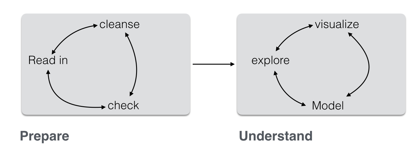
(Inspired by this)

Often, the first major part – “prepare” – is the most time consuming. This can be lamented since many analysts prefer the cool modeling aspects (since I want to show my math!). In practice, one rather has to get his (her) hands dirt…

In this post, I want to put together some kind of checklist of frequent steps in data preparation. More precisely, I would like to detail some typical steps in “cleansing” your data. Such steps include:

• identify missings
• identify outliers
• check for overall plausibility and errors (e.g, typos)
• identify highly correlated variables
• identify variables with (nearly) no variance
• identify variables with strange names or values
• check variable classes (eg. characters vs factors)
• remove/transform some variables (maybe your model does not like categorial variables)
• rename some variables or values (especially interesting if large number)
• check some overall pattern (statistical/ numerical summaries)
• center/scale variables

Don’t get lost in big projects

Before we get in some details, let’s consider some overall guidelines. I have noticed that some projects keep growing like weed, and I find myself bewildered in some jungle… The difficulties then arise not because data or models are difficult, but due to the sheer volume of the analysis.

All in a function

Put analytical steps which belong together in one function. For example, build one function for data cleansing, give as input the raw data frame and let it spit out the processed data frame after all your cleansing steps:

cleansed_data <- cleanse_data(raw_dirty_data,
                              step_01 = TRUE,
                              step_02 = TRUE,
                              step_03 = TRUE)

Although functions are a bit more difficult to debug, at the end of the day it is much easier. Normally or often the steps will be run many times (for different reasons), so it is much easier if all is under one roof.

That said, pragmtic programming suggests to start easy, and to refactor frequently. So better start with a simple solution that works than to have a enormous code that chokes. Get the code running, then improve on it.

Data set for practice

The OKCupid Data set (sanitized version, no names!) is quite nice. You can download it here.

In the following, I will assume that these data are available.

data(profiles, package = "okcupiddata")
data <- profiles

So, the data set is quite huge: 59946, 22 (rows/cols)

Let’s have a brief look at the data.

library(dplyr)
glimpse(data)

## Observations: 59,946
## Variables: 22
## $ age         <int> 22, 35, 38, 23, 29, 29, 32, 31, 24, 37, 35, 28, 24...
## $ body_type   <chr> "a little extra", "average", "thin", "thin", "athl...
## $ diet        <chr> "strictly anything", "mostly other", "anything", "...
## $ drinks      <chr> "socially", "often", "socially", "socially", "soci...
## $ drugs       <chr> "never", "sometimes", NA, NA, "never", NA, "never"...
## $ education   <chr> "working on college/university", "working on space...
## $ ethnicity   <chr> "asian, white", "white", NA, "white", "asian, blac...
## $ height      <int> 75, 70, 68, 71, 66, 67, 65, 65, 67, 65, 70, 72, 72...
## $ income      <int> NA, 80000, NA, 20000, NA, NA, NA, NA, NA, NA, NA, ...
## $ job         <chr> "transportation", "hospitality / travel", NA, "stu...
## $ last_online <dttm> 2012-06-28 20:30:00, 2012-06-29 21:41:00, 2012-06...
## $ location    <chr> "south san francisco, california", "oakland, calif...
## $ offspring   <chr> "doesn't have kids, but might want them", "doesn't...
## $ orientation <chr> "straight", "straight", "straight", "straight", "s...
## $ pets        <chr> "likes dogs and likes cats", "likes dogs and likes...
## $ religion    <chr> "agnosticism and very serious about it", "agnostic...
## $ sex         <chr> "m", "m", "m", "m", "m", "m", "f", "f", "f", "m", ...
## $ sign        <chr> "gemini", "cancer", "pisces but it doesn't matter"...
## $ smokes      <chr> "sometimes", "no", "no", "no", "no", "no", NA, "no...
## $ speaks      <chr> "english", "english (fluently), spanish (poorly), ...
## $ status      <chr> "single", "single", "available", "single", "single...
## $ essay0      <chr> "about me:    i would love to think that i was som...

What’s in a name?

With the code getting longer, it is easy to get confused about naming: data_v2_no_missings_collapsed is the right data matrix to proceed, wasn’t it? Or rather data_dat_edit_noNA_v3? Probably a helpful (though partial) solution is to prevent typing a lot. “Don’t repeat yourself” - if stuff is put inside a function, the objects will not clutter your environment, and you don’t have to deal with them all the time. Also, you will reduce code, and the number of objects if stuff is put inside functions and loops.

That raises the question who to name the data set? At least two points are worth thinking. First, the “root” name should it be the name of the project such as “OKCupid” or “nycflights13”? Or just something like “data”? Personally, I prefer “data” as it is short and everybody will know what’s going on. Second question: Should some data manipulations should be visible in the name of the object? I, personally, like this and do that frequently, eg., carat_mean, so I will remember that the mean is in there. However, for bigger projects I have made the experience that I lose track on which is the most recent version. So better do not put data manipulations in the name of the data frame. However, what one can do is use attributes, eg.:

data_backup <- removing_missings_somehow(data)  # pseudo funtion here for illustration
data <- data_backup

attr(data, "NA_status") <- "no_NA"

Checklist

Clearly, there are different ways to get to Rome; I present just one, which has proved helpful for me.

Identify missings

A key point is here to address many columns in one go, otherwise it gets laborious with large data sets. Here’s one way:

library(knitr)

data %>% 
  summarise_all(funs(sum(is.na(.)))) %>% kable

The function kable prints a html table (package knitr).

There seem to be quite a bit missings. Maybe better plot it.

library(ggplot2)
library(tidyr)

data %>% 
  summarise_all(funs(sum(is.na(.)))) %>% 
  gather %>% 
  ggplot(aes(x = reorder(key, value), y = value)) + geom_bar(stat = "identity") +
  coord_flip() +
  xlab("variable") +
  ylab("Absolute number of missings")

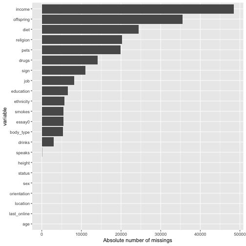
With this large number of missings, we probably will not find an easy solution. Skipping cases will hurt, but imputating may also not be appropriate. Ah, now I know: Let’s just leave it as it is for the moment :-)

Or, at least let’s remember which columns have more than, say, 10%, missings:

cols_with_some_NA <- round(colMeans(is.na(data)),2)
cols_with_too_many_NA <- cols_with_some_NA[cols_with_some_NA > .1]

# alterntively:
data %>% 
  select_if(function(col) mean(is.na(col)) < .1) %>% 
  head

##   age      body_type   drinks           ethnicity height
## 1  22 a little extra socially        asian, white     75
## 2  35        average    often               white     70
## 3  38           thin socially                <NA>     68
## 4  23           thin socially               white     71
## 5  29       athletic socially asian, black, other     66
## 6  29        average socially               white     67
##           last_online                        location orientation sex
## 1 2012-06-28 20:30:00 south san francisco, california    straight   m
## 2 2012-06-29 21:41:00             oakland, california    straight   m
## 3 2012-06-27 09:10:00       san francisco, california    straight   m
## 4 2012-06-28 14:22:00            berkeley, california    straight   m
## 5 2012-06-27 21:26:00       san francisco, california    straight   m
## 6 2012-06-29 19:18:00       san francisco, california    straight   m
##      smokes                                                speaks
## 1 sometimes                                               english
## 2        no english (fluently), spanish (poorly), french (poorly)
## 3        no                                  english, french, c++
## 4        no                              english, german (poorly)
## 5        no                                               english
## 6        no                    english (fluently), chinese (okay)
##      status
## 1    single
## 2    single
## 3 available
## 4    single
## 5    single
## 6    single
##                                                                                                                                         essay0
## 1 about me:    i would love to think that i was some some kind of intellectual: either the dumbest smart guy, or the smartest dumb guy. can't 
## 2 i am a chef: this is what that means.  1. i am a workaholic.  2. i love to cook regardless of whether i am at work.  3. i love to drink and 
## 3 i'm not ashamed of much, but writing public text on an online dating site makes me pleasantly uncomfortable. i'll try to be as earnest as po
## 4                                                                                                    i work in a library and go to school. . .
## 5 hey how's it going? currently vague on the profile i know, more to come soon. looking to meet new folks outside of my circle of friends. i'm
## 6 i'm an australian living in san francisco, but don't hold that against me. i spend most of my days trying to build cool stuff for my company

OK, that are length(cols_with_too_many_NA) columns. We would not want to exclude them because they are too many.

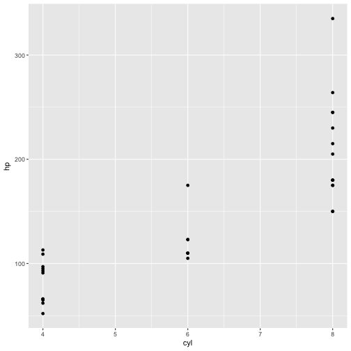
Identify outliers

Obviously, that’s a story for numeric variable only. So let’s have a look at them first.

data %>% 
  select_if(is.numeric) %>% names

## [1] "age"    "height" "income"

Histograms are a natural and easy way to spot them and to learn something about the distribution.

data %>% 
  select_if(is.numeric) %>% 
  gather %>% 
  ggplot(aes(x = value)) + facet_wrap(~ key, scales = "free", nrow = 3) +
  geom_histogram()

## `stat_bin()` using `bins = 30`. Pick better value with `binwidth`.

## Warning: Removed 48445 rows containing non-finite values (stat_bin).

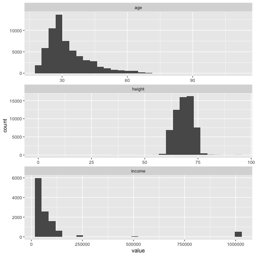
Especially income may be problematic.

Find out more on gather eg., here.

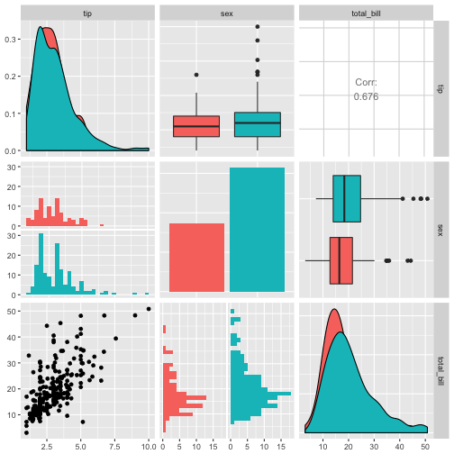
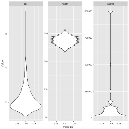
Box plots (or violin plots/bean plots) may also be a way:

data %>% 
  select_if(is.numeric) %>% 
  gather %>% 
  ggplot(aes(x = 1, y = value)) + facet_wrap(~ key, scales = "free") + 
  geom_violin() +
  ylab("Value") +
  xlab("Variable")

## Warning: Removed 48445 rows containing non-finite values (stat_ydensity).

Identify variables with unique values

Similar to outliers, for categorical variable we can look whether some values are seldom, e.g, only 0.1% of the times. What “often” or “barely” is, depends on … you!

library(purrr)

data %>% 
  select_if(negate(is.numeric)) %>% 
  select(-matches("essay")) %>% 
  select(-last_online) %>% 
  gather %>% 
  ggplot(aes(x = value)) + geom_bar() + 
  facet_wrap(~ key, scales = "free", ncol = 3) 

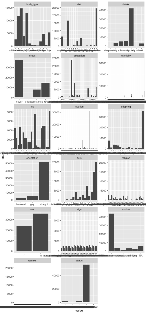
Pooh, that takes ages to plot. And does not look too pretty. Maybe better don’t plot, since we are not after exploration, but just want to know if something is going wrong.

Maybe it is better if we do the following:

for each non-numeric variable do divide most frequent category by least frequent category

This gives an indication whether some categories are quite frequent in relation to others.

data %>% 
  select_if(is.character) %>% 
  summarise_each(funs(max(table(.)/(min(table(.)))))) %>% 
  arrange %>% 
  kable

Plausibility check

Plausibility check can includes checking orders of magnitude, looking for implausible values (negative body weight), among others. A good starter is to differentiate between numeric and non-numeric variables.

Numeric

data %>% 
  select_if(is.numeric) %>% 
  map(summary)

## $age
##    Min. 1st Qu.  Median    Mean 3rd Qu.    Max. 
##   18.00   26.00   30.00   32.34   37.00  110.00 
## 
## $height
##    Min. 1st Qu.  Median    Mean 3rd Qu.    Max.    NA's 
##     1.0    66.0    68.0    68.3    71.0    95.0       3 
## 
## $income
##    Min. 1st Qu.  Median    Mean 3rd Qu.    Max.    NA's 
##   20000   20000   50000  104400  100000 1000000   48442

The function map comes from package purrr; it maps each selected column to the function summary.

For instance, the max. age of 110 appears somewhat high… And the min. height of 1 should rather be excluded before further operations start. For income similar reasoning applies.

Non-numeric

Let’s do not look at all these essay variables here, because “strange” values are not so straight forward to identify compared to more normal categorical variables (with less distinct values).

data %>% 
  select(-matches("essay")) %>% 
  select_if(is.character) %>% 
  mutate_all(factor) %>% 
  map(summary)

Output truncated, TL;DR

We need to convert to factor because for character variables, no nice summary is available of the shelf.

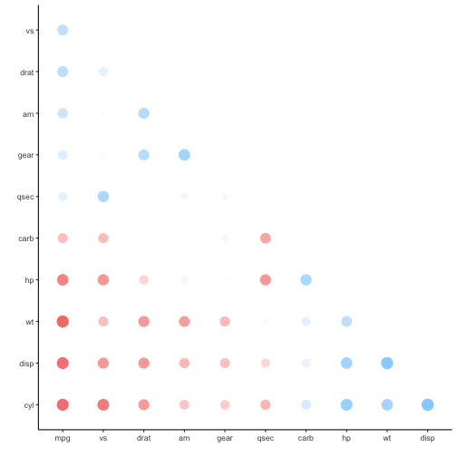
Highly correlated variables

data %>% 
  select_if(is.numeric) %>% 
  cor

##        age height income
## age      1     NA     NA
## height  NA      1     NA
## income  NA     NA      1

Constants/ near zero variance variables

Applies to numeric variables obviously.

data %>% 
  select_if(is.numeric) %>% 
  na.omit %>% 
  summarise_all(c("sd", "IQR"))

##     age_sd height_sd income_sd age_IQR height_IQR income_IQR
## 1 9.746844  4.003725  201433.5      12          5      80000

Rename many variables

ncol_data <- ncol(data) 
names_data_new <- paste("V",1:ncol_data, sep = "")
dummy <- data
names(dummy) <- names_data_new

Recode values

A quite frequent use case is to get “strange” value or variables names in order, e.g., “variable 2” or “I rather not say” (including blanks or some other non-normal stuff).

One approach is to use dplyr::recode.

dplyr::distinct(data, body_type)

##         body_type
## 1  a little extra
## 2         average
## 3            thin
## 4        athletic
## 5             fit
## 6            <NA>
## 7          skinny
## 8           curvy
## 9    full https://sebastiansauer.github.io/images/2017-02-13d
## 10         jacked
## 11 rather not say
## 12        used up
## 13     overweight

dummy <- dplyr::recode(data$body_type, `a little extra` = "1")
unique(dummy)

##  [1] "1"              "average"        "thin"           "athletic"      
##  [5] "fit"            NA               "skinny"         "curvy"         
##  [9] "full https://sebastiansauer.github.io/images/2017-02-13d"   "jacked"         "rather not say" "used up"       
## [13] "overweight"

A second approach is to use base::levels for factors.

dummy <- data$body_type 
dummy <- factor(dummy)
levels(dummy)

##  [1] "a little extra" "athletic"       "average"        "curvy"         
##  [5] "fit"            "full https://sebastiansauer.github.io/images/2017-02-13d"   "jacked"         "overweight"    
##  [9] "rather not say" "skinny"         "thin"           "used up"

levels(dummy) <- 1:12
levels(dummy)

##  [1] "1"  "2"  "3"  "4"  "5"  "6"  "7"  "8"  "9"  "10" "11" "12"

I do not use plyr:mapvalues because plyr can interfere with dplyr (and dplyr seems more helpful to me).

Center/ scale variables

As often, several approaches. One is:

data %>% 
  select_if(is.numeric) %>% 
  scale() %>% 
  head

##             age      height     income
## [1,] -1.0938888  1.67836042         NA
## [2,]  0.2813681  0.42673429 -0.1211069
## [3,]  0.5987351 -0.07391616         NA
## [4,] -0.9880998  0.67705952 -0.4189719
## [5,] -0.3533659 -0.57456662         NA
## [6,] -0.3533659 -0.32424139         NA

base::scale performs a z-transformation of the matrix (like object) given as input.

But wait; one issue is that the data frame now consists of the numeric variables only. We have to manually knit it together with the rest of the party. Not so convenient. Rather, try this:

data %>% 
  select(-matches("essay")) %>% 
  mutate_if(is.numeric, scale) %>% 
  glimpse

## Observations: 59,946
## Variables: 21
## $ age         <dbl> -1.09388884, 0.28136809, 0.59873508, -0.98809985, ...
## $ body_type   <chr> "a little extra", "average", "thin", "thin", "athl...
## $ diet        <chr> "strictly anything", "mostly other", "anything", "...
## $ drinks      <chr> "socially", "often", "socially", "socially", "soci...
## $ drugs       <chr> "never", "sometimes", NA, NA, "never", NA, "never"...
## $ education   <chr> "working on college/university", "working on space...
## $ ethnicity   <chr> "asian, white", "white", NA, "white", "asian, blac...
## $ height      <dbl> 1.67836042, 0.42673429, -0.07391616, 0.67705952, -...
## $ income      <dbl> NA, -0.1211069, NA, -0.4189719, NA, NA, NA, NA, NA...
## $ job         <chr> "transportation", "hospitality / travel", NA, "stu...
## $ last_online <dttm> 2012-06-28 20:30:00, 2012-06-29 21:41:00, 2012-06...
## $ location    <chr> "south san francisco, california", "oakland, calif...
## $ offspring   <chr> "doesn't have kids, but might want them", "doesn't...
## $ orientation <chr> "straight", "straight", "straight", "straight", "s...
## $ pets        <chr> "likes dogs and likes cats", "likes dogs and likes...
## $ religion    <chr> "agnosticism and very serious about it", "agnostic...
## $ sex         <chr> "m", "m", "m", "m", "m", "m", "f", "f", "f", "m", ...
## $ sign        <chr> "gemini", "cancer", "pisces but it doesn't matter"...
## $ smokes      <chr> "sometimes", "no", "no", "no", "no", "no", NA, "no...
## $ speaks      <chr> "english", "english (fluently), spanish (poorly), ...
## $ status      <chr> "single", "single", "available", "single", "single...

If we only want to center (or something similar), we could do

data %>% 
  mutate_if(is.numeric, funs(. - mean(.))) %>% 
  head

##         age      body_type              diet   drinks     drugs
## 1 -10.34029 a little extra strictly anything socially     never
## 2   2.65971        average      mostly other    often sometimes
## 3   5.65971           thin          anything socially      <NA>
## 4  -9.34029           thin        vegetarian socially      <NA>
## 5  -3.34029       athletic              <NA> socially     never
## 6  -3.34029        average   mostly anything socially      <NA>
##                           education           ethnicity height income
## 1     working on college/university        asian, white     NA     NA
## 2             working on space camp               white     NA     NA
## 3    graduated from masters program                <NA>     NA     NA
## 4     working on college/university               white     NA     NA
## 5 graduated from college/university asian, black, other     NA     NA
## 6 graduated from college/university               white     NA     NA
##                              job         last_online
## 1                 transportation 2012-06-28 20:30:00
## 2           hospitality / travel 2012-06-29 21:41:00
## 3                           <NA> 2012-06-27 09:10:00
## 4                        student 2012-06-28 14:22:00
## 5    artistic / musical / writer 2012-06-27 21:26:00
## 6 computer / hardware / software 2012-06-29 19:18:00
##                          location                              offspring
## 1 south san francisco, california doesn't have kids, but might want them
## 2             oakland, california doesn't have kids, but might want them
## 3       san francisco, california                                   <NA>
## 4            berkeley, california                      doesn't want kids
## 5       san francisco, california                                   <NA>
## 6       san francisco, california doesn't have kids, but might want them
##   orientation                      pets
## 1    straight likes dogs and likes cats
## 2    straight likes dogs and likes cats
## 3    straight                  has cats
## 4    straight                likes cats
## 5    straight likes dogs and likes cats
## 6    straight                likes cats
##                                   religion sex
## 1    agnosticism and very serious about it   m
## 2 agnosticism but not too serious about it   m
## 3                                     <NA>   m
## 4                                     <NA>   m
## 5                                     <NA>   m
## 6                                  atheism   m
##                           sign    smokes
## 1                       gemini sometimes
## 2                       cancer        no
## 3 pisces but it doesn't matter        no
## 4                       pisces        no
## 5                     aquarius        no
## 6                       taurus        no
##                                                  speaks    status
## 1                                               english    single
## 2 english (fluently), spanish (poorly), french (poorly)    single
## 3                                  english, french, c++ available
## 4                              english, german (poorly)    single
## 5                                               english    single
## 6                    english (fluently), chinese (okay)    single
##                                                                                                                                         essay0
## 1 about me:    i would love to think that i was some some kind of intellectual: either the dumbest smart guy, or the smartest dumb guy. can't 
## 2 i am a chef: this is what that means.  1. i am a workaholic.  2. i love to cook regardless of whether i am at work.  3. i love to drink and 
## 3 i'm not ashamed of much, but writing public text on an online dating site makes me pleasantly uncomfortable. i'll try to be as earnest as po
## 4                                                                                                    i work in a library and go to school. . .
## 5 hey how's it going? currently vague on the profile i know, more to come soon. looking to meet new folks outside of my circle of friends. i'm
## 6 i'm an australian living in san francisco, but don't hold that against me. i spend most of my days trying to build cool stuff for my company

That’s it; happy analyzing!