Let’s plot some skewed stuff, aehm, distributions!

Actually, the point I - initially - wanted to make is that in skewed distribution, don’t use means. Or at least, be very aware that (arithmetic) means can be grossly misleading. But for today, let’s focus on drawing skewed distributions.

Some packages:

library(tidyverse)
library(fGarch) # for snorm

Some skewed distribution include:

• “polluted” normal distributions, ie., mixtures of two normals
• Exponential distributions
• Gamma distributions
• Beta distributions

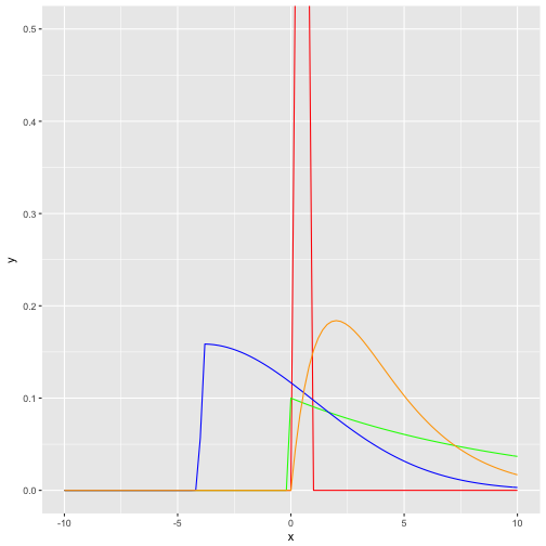
One way to visualize them is to draw their curve, ie., their functional (analytical) form:

data_frame(
  x = seq(-10, 10, .05)
) %>% 
  ggplot +
  aes(x) +
  stat_function(fun = dbeta, args = list(shape1 = 4, shape2 = 4), color = "red") +
  stat_function(fun = dexp, args = list(rate = .10), color = "green") +
  stat_function(fun = dsnorm, args = list(mean = 0, sd = 3, xi = 7.5), color = "blue") +
  stat_function(fun = dgamma, args = list(shape = 2, scale = 2), color = "orange") +
  coord_cartesian(ylim = c(0,.5))

Second, we could draw some random instances from the respective distribution; we will get then not “smooth” curves but more “realistic” or “zigzag” histogram (or density diagrams).

df <- data_frame(
  skewed_normal = rsnorm(n = 1000, mean = 0, sd = 18, xi = 130),
  exp_distrib = rexp(n = 1000, rate = .1),
  gamma_distrib = rgamma(n = 1000, shape = 2, scale = 2),
  beta_distrib = rbeta(n = 1000, shape1 = 4, shape2 = 2)
  
)

mypal <- 

df %>% 
  gather(key = distribution, value = value) %>% 
  ggplot +
  aes(x = value) +
  geom_histogram(aes(fill = distribution)) +
  facet_wrap(~distribution) +
  scale_fill_manual(values = c("red", "green", "blue", "orange")) +
  scale_color_manual(values = c("red", "green", "blue", "orange")) +
  labs(title = "Histogram of random draws from different distributions",
       subtitle = "test")

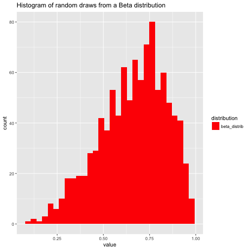
Note that the domain of the beta distribution is [0,1], that’s why a narrow red bar pops out as histogram (the other distribution spread out much more explicitly). See:

df %>% 
  gather(key = distribution, value = value) %>% 
  dplyr::filter(distribution == "beta_distrib") %>% 
  ggplot +
  aes(x = value) +
  geom_histogram(aes(fill = distribution)) +
  #facet_wrap(~distribution) +
  scale_fill_manual(values = c("red", "green", "blue", "orange")) +
  scale_color_manual(values = c("red", "green", "blue", "orange")) +
  labs(title = "Histogram of random draws from a Beta distribution")

## `stat_bin()` using `bins = 30`. Pick better value with `binwidth`.

Moderator effects (ie., interaction or synergy effects) are a topic of frequent interest in many sciences braches. A lot ink has been spilled over this topic (so did I, eg., here).

However, in that post I did now show how to visualize error in case of nominal (categorical) independent variable, and categorical moderator.

Luckily, visualization of this case is quite straight forward with ggplot2.

First, some data and packages to be loaded:

library(tidyverse)
data(tips, package = "reshape2")

Then, we summarise the data:

tips %>% 
  group_by(sex, smoker) %>% 
  summarise(tip_groups = mean(tip),
            tip_sem = (sd(tip)/sqrt(length(tip)))) -> tips2
tips2

## Source: local data frame [4 x 4]
## Groups: sex [?]
## 
##      sex smoker tip_groups tip_sem
##   <fctr> <fctr>      <dbl>   <dbl>
## 1 Female     No       2.77   0.154
## 2 Female    Yes       2.93   0.212
## 3   Male     No       3.11   0.151
## 4   Male    Yes       3.05   0.194

Remember that the standard error of the mean is computed as

\(sem = \frac{sd(x)}{\sqrt{n}}\) Now we take this summarised data and plot it:

tips2 %>% 
  ggplot() +
  aes(x = sex, y = tip_groups, color = smoker) +
  geom_line(aes(group = smoker)) +
  geom_point() +
  geom_linerange(aes(x = sex, ymin = tip_groups - tip_sem, ymax = tip_groups + tip_sem), size = .3) +
  labs(title = "Moderating role of smoking status on the effect of sex on tip",
       subtitle = "Error bars indicate standard error of the mean")

Maybe better changing the domain of the y-axis to put the effects in a (different) perspective:

tips2 %>% 
  ggplot() +
  aes(x = sex, y = tip_groups, color = smoker) +
  geom_line(aes(group = smoker)) +
  geom_point() +
  geom_linerange(aes(x = sex, ymin = tip_groups - tip_sem, ymax = tip_groups + tip_sem), size = .3) +
  labs(title = "Moderating role of smoking status on the effect of sex on tip",
       subtitle = "Error bars indicate standard error of the mean") +
  scale_y_continuous(limits = c(0,5))

It is well-known that the notorious p-values is sensitive to sample size: The larger the sample, the more bound the p-value is to fall below the magic number of .05.

Of course, the p-value is also a function of the effect size, eg., the distance between two means and the respective variances. But still, the p-values tends to become significant in the face of larges samples, and non-significant otherwise.

Theoretically, quite simple and well understood. But let’s take the test of “real” data and do a simulation to demonstrate or test this behavior.

First, load some required packages

library(tidyverse)

Simulate data with large sample size

Next, we simulate data: A data frame of 20 cols and many rows (1e06, ie., 1 million). We should also make sure that the null hypothesis is false in our data. To that end, we let the mean values of the columns vary somewhat.

k <- 20
n <- 1e06
df <- data.frame(replicate(k,rnorm(n = n, mean = rnorm(1, 0, 1), sd = 1)))

Now let’s compute t-tests for each and every combination (cartesian product of all combinations). We will save the resulting p-values in a (square) matrix.

m <- matrix(nrow = k, ncol = k)


for (i in seq_len(ncol(df))) {
  for (j in seq_len(ncol(df))) {
    m[i, j] <- t.test(df[i], df[j])$p.value
  }
}

One half of the matrix is redundant, as the matrix is symmetric. The same reasoning applies for the diagonal. Let’s take out the redundant elements.

m[lower.tri(m)] <- NA
m[diag(m)] <- NA

Let’s come up with a logical matrix indicating whether one cell (ie., one t-test) indicates a significant t-test (TRUE) or not (FALSE).

m_significant <- apply(m, c(1,2), function(x) x < .05)

Finally, let’s count the number of significant results, and sum then up.

m_significant %>% sum(TRUE, na.rm = TRUE)

## [1] 191

The number of different tests is \((k*k - k)/2\).

Which amounts, in this case to

(k*k-20)/2

## [1] 190

Hence, all tests are significant.

rm(df)

Simulate data with small sample size

Now, we repeat the same thing with a small sample.

simulate_ps <- function(n = 1e06, k = 20){
  
  # arguments:
  # n: number of rows
  # k: number of columns
  # returns: proportion of significant (p<.05) t-tests

set.seed(42)  
  
# simulate data
df <- data.frame(replicate(k,rnorm(n = n, mean = rnorm(1, 0, 1), sd = 1)))

# matrix for t-test results
m <- matrix(nrow = k, ncol = k)

# cartesian product of all t-tests
for (i in seq_len(ncol(df))) {
  for (j in seq_len(ncol(df))) {
    m[i, j] <- t.test(df[i], df[j])$p.value
  }
}

# take-out redundant cells
m[lower.tri(m)] <- NA
m[diag(m)] <- NA

# compute matrix to count number of significant t-tests
m_significant <- apply(m, c(1,2), function(x) x < .05)


# count
sum_significant <- m_significant %>% sum(TRUE, na.rm = TRUE)

sum_distinct_tests <- (k*k - k)/2

prop_significant <- sum_significant / sum_distinct_tests

rm(df)
return(prop_significant)

}

simulate_ps(n = 10, k = 20)

## [1] 0.5894737

Play around

Now, we can play around a bit.

ns <- c(5, 10, 15, 20, 30, 40, 50, 100, 200, 300, 500, 1000, 2000, 5000, 10000, 2e04, 5e04, 1e05)

ps <- vector(mode = "numeric", length = length(ns))

for (i in seq_along(ns)){
  ps[i] <- simulate_ps(n = ns[i], k = 20)
  print(ps[i])
}

## [1] 0.4263158
## [1] 0.5894737
## [1] 0.5789474
## [1] 0.7315789
## [1] 0.6473684
## [1] 0.7736842
## [1] 0.8368421
## [1] 0.8631579
## [1] 0.9473684
## [1] 0.8842105
## [1] 0.9157895
## [1] 0.9736842
## [1] 0.9894737
## [1] 0.9894737
## [1] 0.9947368
## [1] 0.9947368
## [1] 1
## [1] 0.9947368

Finally, let’s plot that:

data_frame(
  ns = ns,
  ps = ps
)  %>% 
  ggplot +
  aes(x = ns, y = ps) +
  geom_line(color = "gray80") +
  geom_point(color = "firebrick")

Thus, our result appears reasonable: The larger the sample size (ns), the higher the proportion of ps (ps).

Dichotomizing is also called dummy coding. It means: Take a variable with multiple different values (>2), and transform it so that the output variable has 2 different values.

Note that this “thing” can be understood as consisting of two different aspects: Recoding and cutting. Recoding means that value “a” becomes values “b” etc. Cutting means that a “rope” of numbers is cut into several shorter “ropes” (that’s why it is called cutting).

Several ways of achieving this exist in R. Here we discuss three.

First, let’s load some data.

library(AER)
data(Affairs)

We will define a new variable, called “halodrie”. A “halodrie” is someone who likes having affairs (German parlance). The variable should have 2 values, ie., “yes” and “no”.

Using {car}

library(car)

Affairs$halodrie <- car::recode(Affairs$affairs, "0 = 'no'; 1:12 = 'yes'")

head(Affairs$halodrie)

## [1] "no" "no" "no" "no" "no" "no"

table(Affairs$halodrie)

## 
##  no yes 
## 451 150

A comfortable feature of this function is that it allows using the colon operator. Note that the whole recode-thing (all values to be recoded) is to be put into quotation marks.

Using {dplyr}

library(dplyr)

Affairs$halodrie <- 
  dplyr::recode(Affairs$affairs, `0` = "no", .default = "yes")

Affairs$halodrie %>% head

## [1] "no" "no" "no" "no" "no" "no"

table(Affairs$halodrie)

## 
##  no yes 
## 451 150

This function does not allow the colon operator. I assume the reason that the author (Hadley Wickham) argues that a given function should only be capable of one thing. Here, the function reassigns a value of a variable, not (much) more, not less.

Using base::cut

Affairs$halodrie <- cut(Affairs$affairs, breaks = c(-Inf, 0, +Inf), labels = c("no", "yes"))

table(Affairs$halodrie)

## 
##  no yes 
## 451 150

Of note, when a continuous variable is “cut”, one must specify the minimum and the maximum value (or arbitrarly small or large values) as cutting points. So cutting in two halfs, is not one cutting point for cut, but three (always add two cutting points: one being the smallest value in the sample [or smaller, even -Inf, the other one being the largest value in the sample [or even Inf]).

Summary

For beginners, I would recommend car::recode. It provides both recoding and cutting in one function, and hence may be easier to apply at start. It also offers quite some flexibility. Assume you are interested in marriages ranging from 5 to 15 years:

Affairs$years5_15 <- car::recode(Affairs$yearsmarried, "0:4 =  'no'; 5:15 = 'yes'; else = 'no'")

head(Affairs$years5_15)

## [1] "yes" "no"  "yes" "yes" "no"  "no"

table(Affairs$years5_15)

## 
##  no yes 
## 245 356

R thinks columnwise, not rowwise, at least in standard dataframe operations. A typical rowwise operation is to compute row means or row sums, for example to compute person sum scores for psychometric analyses.

One workaround, typical for R, is to use functions such as apply (and friends).

However, dplyr offers some quite nice alternative:

library(dplyr)

mtcars %>% 
  rowwise() %>% 
  mutate(mymean=mean(c(cyl,mpg))) %>% 
  select(cyl, mpg, mymean)

## Source: local data frame [32 x 3]
## Groups: <by row>
## 
## # A tibble: 32 × 3
##      cyl   mpg mymean
##    <dbl> <dbl>  <dbl>
## 1      6  21.0  13.50
## 2      6  21.0  13.50
## 3      4  22.8  13.40
## 4      6  21.4  13.70
## 5      8  18.7  13.35
## 6      6  18.1  12.05
## 7      8  14.3  11.15
## 8      4  24.4  14.20
## 9      4  22.8  13.40
## 10     6  19.2  12.60
## # ... with 22 more rows