Plotting a normal distribution is something needed in a variety of situation: Explaining to students (or professors) the basic of statistics; convincing your clients that a t-Test is (not) the right approach to the problem, or pondering on the vicissitudes of life…

If you like ggplot2, you may have wondered what the easiest way is to plot a normal curve with ggplot2?

Here is one:

library(cowplot)
## Loading required package: ggplot2
## 
## Attaching package: 'cowplot'
## The following object is masked from 'package:ggplot2':
## 
##     ggsave
p1 <- ggplot(data = data.frame(x = c(-3, 3)), aes(x)) +
  stat_function(fun = dnorm, n = 101, args = list(mean = 0, sd = 1)) + ylab("") +
  scale_y_continuous(breaks = NULL)
p1

Note that cowplot here is optional, and gives a more “clean” appearance to the plot. Without cowplot, ie., the standard theme of ggplot2, you will get (better restart your R session before running the next code):

library(ggplot2)


p1 <- ggplot(data = data.frame(x = c(-3, 3)), aes(x)) +
  stat_function(fun = dnorm, n = 101, args = list(mean = 0, sd = 1)) + ylab("") +
  scale_y_continuous(breaks = NULL)
p1

Pearson’s correlation is a well-known and widely used instrument to gauge the degree of linear association of two variables (see this post for an intuition on correlation).

There a many formulas for correlation, but a short and easy one is this one:

.

In words, can be seen as the average product of z-scores.

In “raw values”, r is given by

.

Here, refers to the difference of a value to its mean.

At times it is helpful to write r so that the similarity to the covariance gets clear:

OK. But why is it, that r cannot be larger than 1 (and not smaller than -1)?

That is, why does the following inequality hold: ?

This is the question we are addressing in this post. I haven’t found much on that on the net, so that’s why I sum up some thoughts in this post.

Cauchy-Schwarz Inequality

One explanation, quite straight forward, is based on the Cauchy-Schwarz Inequality. This inequality can be stated as follows:

,

where denotes the dot product of a vector, eg. x.

This formula can be rewritten as

But this formula looks very similar to the correlation, if we first take the square root of both sides:

and then cancel out the (1/n) part from the raw values equation of r above:

.

Now rewrite r in this way:

.

The raw formula of r matches now the Cauchy-Schwarz inequality! Thus, the nominator of r raw formula can never be greater than the denominator. In other words, the whole ratio can never exceed an absolute value of 1.

Looking at the regression line

A second line of reasoning why r cannot the greater than 1 (less than -1) is the following.

Suppose X and Y are perfectly correlated, for example like this:

x <- runif(n = 100, min = 0, max = 10)
res <- rnorm(n = 100)
y <- x
library(ggplot2)
library(tibble)
ggplot(tibble(x, y), aes(x = x, y = y)) + geom_point(alpha = .5)

Now, what happens if we z-scale X and Y? Not much:

z_x <- as.numeric(scale(x))
z_y <- as.numeric(scale(y))

df1 <- tibble(z_x, z_y)
ggplot(df1, aes(x = z_x, y = z_y)) + geom_point(alpha = .5)

The difference is that mean X and meany Y is both zero, and SD for both X and Y is 1, so the scaling has changed (the line has a gradient of 1 now).

Note that perfect correlation of z-scaled variables means that for each there is an of same value.

For example:

library(magrittr)
z_x <- x %>%  scale %>% as.numeric %>% sort
z_y <- y %>%  scale %>% as.numeric %>% sort
df2 <- tibble(z_x, z_y)
head(df2)
## # A tibble: 6 x 2
##         z_x       z_y
##       <dbl>     <dbl>
## 1 -1.688960 -1.688960
## 2 -1.688875 -1.688875
## 3 -1.685675 -1.685675
## 4 -1.621873 -1.621873
## 5 -1.554167 -1.554167
## 6 -1.532031 -1.532031

But if for all X and Y it means that the means and variances of X and Y are the same, too. It actually means that X equals Y.

If we look at the formula of the correlation for perfectly correlated z-scaled variables X and Y we find:

In words, when two variables are perfectly correlated (ie., their graph is a line), then r=1.

This article has been published at The Winnower, it is distributed under the terms of the Creative Commons Attribution 4.0 International License, which permits unrestricted use, distribution, and redistribution in any medium, provided that the original author and source are credited.

Data can be accessed here.

Access the paper here.

CITATION: Sebastian Sauer, Alexander Wolff, The effect of a status symbol on success in online dating: an experimental study (data paper), The Winnower 3:e147241.13309 (2016). DOI: 10.15200/winn.147241.13309


ABSTRACT

volutionary psychology suggests that women and men differ in their mating strategies. We operationalized a central claim of evolutionary psychology by manipulating social status of profiles at a dating website: one group of profiles was depicted with a luxury sports car (high status) and second group without car (low status). Six profile were set up (3 female, 3 male) for each of the two groups. Two type of response variables were collected: Whether a “match” occurred (n=3515), and whether a message was sent to the profile (n=1548). Beauty and hip-waist-ratio of straw persons, and age of contacting individuals were recorded. Given strong effect sizes, large sample size, and high interest in human mating, this data set should be of interest for applied researchers in human mating and social psychology.

BACKGROUND

A central claim of evolutionary psychology is that social status has a positive impact on female mating strategy; men exhibiting higher social status are expected to attract more women compared to men with lower social status (Buss 2015). Social status can be defined as the relative social position an individual is perceived to possess; social status refers to the estimation or status attributed to this position (Coie, Dodge, and Coppotelli 1982). The variety of social status indicators includes income, wealth, social power, social esteem of a social role, or educational level. These effects are well known and widely replicated (Buss et al. 2001).

It has been noted that social status, and particularly wealth, is not only for present times and western women a central mating criterion; this preference has been documented in non-western cultures and different times as well. For example, between 1984 and 1989, Buss and colleagues investigated more than 30 cultures around the globe regarding mating preferences. In sum, approx. 10,000 individuals were included in the study, stemming from six continents (Buss et al. 1990; Buss 1989). Results suggest the importance of male financial situation for women’s mating decisions is an intercultural constant.

The theoretical basis for this behavior is theorized as stemming from the different biological fabric of the sexes. In all mammals, males produce much more sperms than female produce ova. Thus, there should be an incentive for females to prefer males with an outlook of secure breeding of the offspring. Social status and in particular financial wealth are widely viewed as predictors of such reproductive success (Buss 2009; Buss 2015). It should be noted that evolution theory suggests that (mating) mechanisms which are active in inter- or intra-sexual selection have developed in extensive time spans, and cannot quickly accommodate to recent environmental changes, e.g. those of modern human culture. This fact may explain why some strategies appear maladaptive for modern life.

Similarly, it has been suggested that women should prefer men who are slightly older then themselves (Buss 2015). This can be explained by the fact than older men normally possess higher social status (e.g. income) compared to younger men. The present data set allows for testing this hypothesis too.

Apart from social status, physical attractiveness has been proposed as an important (positive) predictor for mating success. One explanation for the relevance of beauty is that beauty may be indicative of health (Shackelford and Larsen 1997; Grammer and Thornhill 1994). Thus, more attractive individuals should attract more partners; this is expected for both sexes, but is maybe more pronounced in the selection process of men (Buss 2015; Abramson 1995). One widely used measure for attractiveness and reproductive outlook is the waist-hip-ratio (Streeter and McBurney 2003; Singh and Young 1995). The present data allow for testing the impact of beauty of mating success.

METHODS

### SAMPLE The sample consists of 3515 matches and 1515 messages; in sum, this behavior originated from n = 1920 individuals in total. There are no missings in the data, as all data were collected electronically. Data are anonymized using a hash mechanism (sha256). Mean age was 29.5 years (sd = 5.0 years). Six straw persons were included in the study, each with a profile with luxury car (high status), and without car (low status), yielding a total of 12 profiles on the dating portal. Of all matches, 3205 (91%) were sent to one of the 6 female profiles; of all messages sent, 310 (98%) were sent to a female profile. It should be noted that participants were matched to the experimental factor by chance alone; the allocation was not counterbalanced in any way due to technical/practical constraints of the dating portal. Data was collected between 2015-01-05 and 2016-01-20.

MATERIALS

The main stimulus was the profile picture. Between the two groups of the experimental factor (“car”), the only difference was whether the luxury car (BMW Z4) was present or not (i.e., high vs. low status). To better control for idiosyncrasies of the straw person (eg. attractiveness), 3 different straw persons of each sex were included. Theses six individuals differed in their subjective attractiveness as judged by a rating committee of five persons on a scale from 1 to 10 (M = 5.8; sd = 1.2) and in their waist-hip-ratio (whr; female: M = 0.71; sd = 0.02; male M = 0.91; sd = 0.02). For reasons of personal rights and privacy, pictures of the straw persons are not made public.

For the names of each straw person, typical German names were chosen (female: “Julia”; men: “Christian”). Year of birth was documented as 1987 for each straw person. No family names were shown. As location, “München” (Germany) was specified. In order to make the profiles of the straw persons more realistic, some typical hobbies were filled in: TV series, music, sports, telephoning with friends.

PROCEDURES

The profiles were setup at one of the largest online dating portals (Germany version) with more than 300 million users (as of Aug. 2016).

The dating portal allowed for checking for “matches”, defined were both individuals judge their counterpart as “interesting” thereby communicating principal interest in further interaction. For each of the 12 profiles, we judged the first 600 user profiles that were suggested by the portal as “interesting”. Each of our profiles was online for one week (no overlaps between the two groups). No further contact was undertaken with the individuals contacting our straw persons; in particular, we did not respond to any matching or contact message.

Man icon made by Freepik from www.flaticon.com is licensed by CC 3.0 BY

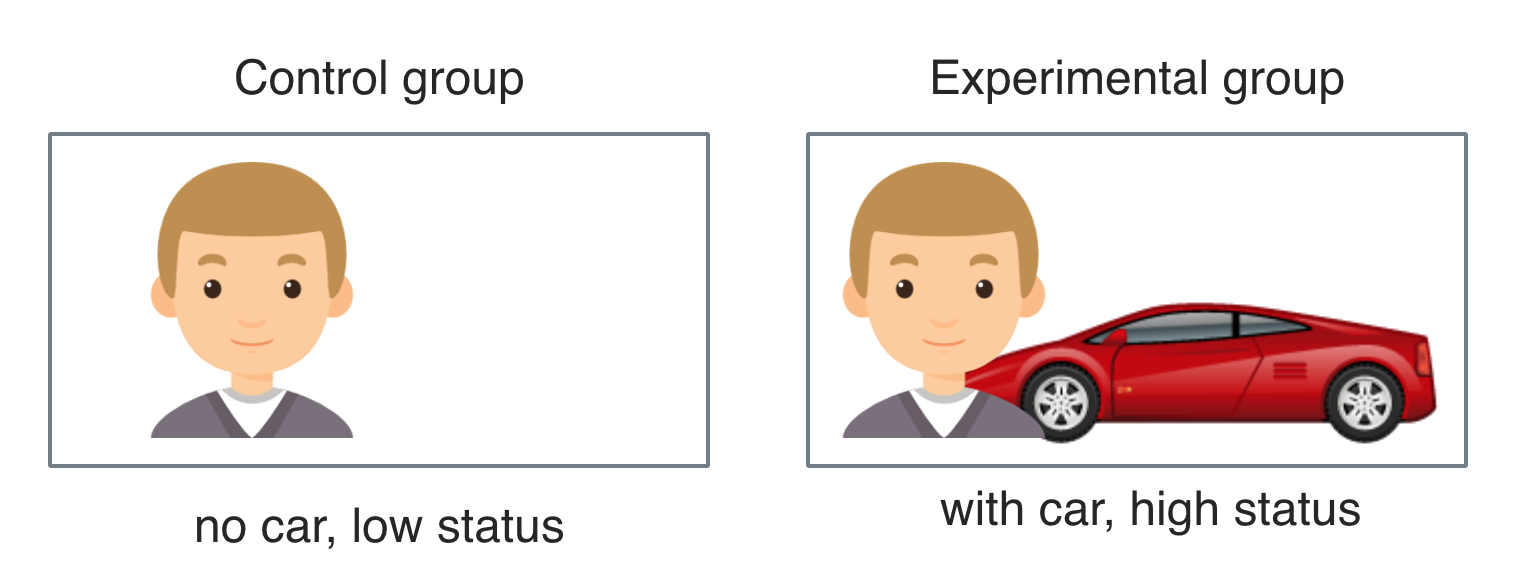
Car icon made by IconShow is licenced for non-commercial use.

Data was collected electronically by the portal, so it can be expected that no typos or similar errors are present in the data. We performed some “sanity checks”, e.g. checked whether all values are plausible. Finally, we checked that the anonymization had worked. No errors or quality restrictions were identified.

ETHICAL ISSUES

This study was part of a MSc thesis, and was approved by the supervising professor (disclaimer: the supervising professor is one of the authors). As we did not engage in any contact with the individuals contacting our straw persons it appears unlikely that strong emotions and strong negative affect occurred. We did not receive any signs of discontent from the participants. No further debriefing took place. We declare that we have no conflicts of interest.

DATASET DESCRIPTION

### Object name

data

Data type

primary data (anonymized)

Format names and versions

CSV

Language

English

Licence

CC-BY-4

Embargo

none

Repository location

http://www.osf.io/4hkjm

Publication date at reposository

2016-08-17

Dimensions of data set

5063 observations of 9 variables. See codebook for details.

Reuse potential

The data set allows for testing (replicating) some of the main claims of evolutionary psychology with regard to human mating. The results of the present data have not been published yet; given the strong effects, the large sample size and the high overall interest in evolutionary psychology in general and human mating in particular, this data set can be expected to be of substantial interest. Additional, refined analysis, aggregation to existing bodies of data, and teaching (due to the general “lay” interest) are included in potential reuses of this data set.

ACKNOWLEDGEMENTS

None.

REFERENCES

Abramson, Paul R. 1995. Sexual Nature/sexual Culture. University of Chicago Press.

Buss, David M. 1989. “Sex Differences in Human Mate Preferences: Evolutionary Hypotheses Tested in 37 Cultures.” Behavioral and Brain Sciences 12 (01). Cambridge Univ Press: 1–14.

———. 2009. “The Great Struggles of Life: Darwin and the Emergence of Evolutionary Psychology.” American Psychologist 64 (2). American Psychological Association: 140.

———. 2015. Evolutionary Psychology: The New Science of the Mind. Psychology Press.

Buss, David M, Max Abbott, Alois Angleitner, Armen Asherian, Angela Biaggio, Angel Blanco-Villasenor, M Bruchon-Schweitzer, et al. 1990. “International Preferences in Selecting Mates a Study of 37 Cultures.” Journal of Cross-Cultural Psychology 21 (1). Sage Publications: 5–47.

Buss, David M, Todd K Shackelford, Lee A Kirkpatrick, and Randy J Larsen. 2001. “A Half Century of Mate Preferences: The Cultural Evolution of Values.” Journal of Marriage and Family 63 (2). Wiley Online Library: 491–503.

Coie, John D, Kenneth A Dodge, and Heide Coppotelli. 1982. “Dimensions and Types of Social Status: A Cross-Age Perspective.” Developmental Psychology 18 (4). American Psychological Association: 557.

Grammer, Karl, and Randy Thornhill. 1994. “Human (Homo Sapiens) Facial Attractiveness and Sexual Selection: The Role of Symmetry and Averageness.” Journal of Comparative Psychology 108 (3). American Psychological Association: 233.

Shackelford, Todd K, and Randy J Larsen. 1997. “Facial Asymmetry as an Indicator of Psychological, Emotional, and Physiological Distress.” Journal of Personality and Social Psychology 72 (2). American Psychological Association: 456.

Singh, Devendra, and Robert K Young. 1995. “Body Weight, Waist-to-Hip Ratio, Breasts, and Hips: Role in Judgments of Female Attractiveness and Desirability for Relationships.” Ethology and Sociobiology 16 (6). Elsevier: 483–507.

Streeter, Sybil A, and Donald H McBurney. 2003. “Waist–hip Ratio and Attractiveness: New Evidence and a Critique of a Critical Test.” Evolution and Human Behavior 24 (2). Elsevier: 88–98.

t-Test on multiple columns

Suppose you have a data set where you want to perform a t-Test on multiple columns with some grouping variable. As an example, say you a data frame where each column depicts the score on some test (1st, 2nd, 3rd assignment…). In each row is a different student. So you glance at the grading list (OMG!) of a teacher!

How to do do that in R? Probably, the most “natural” solution would be some lapply() call.

But I like dplyr (see intro here); so, is there some nice way to perform that with dplyr? The short answer is: no. dplyr basically wants to deliver back a data frame, and the t-test does not output a single value, so you cannot use the t-test (right away) for dplyr’s summarise. One way out is using list-columns… Let’s see.

Load some dplyr, tidyr and some data:

library(dplyr)
library(tidyr)
data(tips, package = "reshape2")
glimpse(tips)
## Observations: 244
## Variables: 7
## $ total_bill <dbl> 16.99, 10.34, 21.01, 23.68, 24.59, 25.29, 8.77, 26....
## $ tip        <dbl> 1.01, 1.66, 3.50, 3.31, 3.61, 4.71, 2.00, 3.12, 1.9...
## $ sex        <fctr> Female, Male, Male, Male, Female, Male, Male, Male...
## $ smoker     <fctr> No, No, No, No, No, No, No, No, No, No, No, No, No...
## $ day        <fctr> Sun, Sun, Sun, Sun, Sun, Sun, Sun, Sun, Sun, Sun, ...
## $ time       <fctr> Dinner, Dinner, Dinner, Dinner, Dinner, Dinner, Di...
## $ size       <int> 2, 3, 3, 2, 4, 4, 2, 4, 2, 2, 2, 4, 2, 4, 2, 2, 3, ...

Well, it looks crude, but that’s a way:

tips %>% 
  select(tip, total_bill, sex) %>% 
  gather(key = variable, value = value, -sex) %>% 
  group_by(sex, variable) %>% 
  summarise(value = list(value)) %>% 
  spread(sex, value) %>% 
  group_by(variable) %>% 
  mutate(p_value = t.test(unlist(Female), unlist(Male))$p.value,
         t_value = t.test(unlist(Female), unlist(Male))$statistic)
## Source: local data frame [2 x 5]
## Groups: variable [2]
## 
##     variable     Female        Male    p_value   t_value
##        <chr>     <list>      <list>      <dbl>     <dbl>
## 1        tip <dbl [87]> <dbl [157]> 0.13780684 -1.489536
## 2 total_bill <dbl [87]> <dbl [157]> 0.01857339 -2.373398

Let’s go through this code step by step. First, this bit

tips %>% 
  select(tip, total_bill, sex) %>% head
##    tip total_bill    sex
## 1 1.01      16.99 Female
## 2 1.66      10.34   Male
## 3 3.50      21.01   Male
## 4 3.31      23.68   Male
## 5 3.61      24.59 Female
## 6 4.71      25.29   Male

is used to select the columns we want to perform the t-Test on (here: tip and total_bill) plus the grouping variable (sex).

Then by the next bit

tips %>% 
  select(tip, total_bill, sex) %>% 
  gather(key = variable, value = value, -sex) %>% head
##      sex variable value
## 1 Female      tip  1.01
## 2   Male      tip  1.66
## 3   Male      tip  3.50
## 4   Male      tip  3.31
## 5 Female      tip  3.61
## 6   Male      tip  4.71

we “melt” the data frame down, so that all numeric variables are put in one column (underneath each other).

tips %>% 
  select(tip, total_bill, sex) %>% 
  gather(key = variable, value = value, -sex) %>% 
  group_by(sex, variable) %>% 
  summarise(value = list(value)) 
## Source: local data frame [4 x 3]
## Groups: sex [?]
## 
##      sex   variable       value
##   <fctr>      <chr>      <list>
## 1 Female        tip  <dbl [87]>
## 2 Female total_bill  <dbl [87]>
## 3   Male        tip <dbl [157]>
## 4   Male total_bill <dbl [157]>

Now it get’s interesting. We put all the values per group (e.g., male-tip or female-total_bill…) in one cell. Yes, that’s right. In each cell of column value there is now a list (a bunch) of values. That’s what is called a “list-column”. We will now use this list column for the t-test.

tips %>% 
  select(tip, total_bill, sex) %>% 
  gather(key = variable, value = value, -sex) %>% 
  group_by(sex, variable) %>% 
  summarise(value = list(value)) %>% 
  spread(sex, value) %>% 
  group_by(variable) 
## Source: local data frame [2 x 3]
## Groups: variable [2]
## 
##     variable     Female        Male
## *      <chr>     <list>      <list>
## 1        tip <dbl [87]> <dbl [157]>
## 2 total_bill <dbl [87]> <dbl [157]>

But before we do the t-Test, we “spread” the data frame. That is, we convert from “long” to “wide” format. Next, we group for variable. That means in practice, that the following t-test will be applied to each member of this group (ie., each variable, here tip and total_bill).

And now the t-Test:

tips %>% 
  select(tip, total_bill, sex) %>% 
  gather(key = variable, value = value, -sex) %>% 
  group_by(sex, variable) %>% 
  summarise(value = list(value)) %>% 
  spread(sex, value) %>% 
  group_by(variable) %>% 
  mutate(p_value = t.test(unlist(Female), unlist(Male))$p.value,
         t_value = t.test(unlist(Female), unlist(Male))$statistic)
## Source: local data frame [2 x 5]
## Groups: variable [2]
## 
##     variable     Female        Male    p_value   t_value
##        <chr>     <list>      <list>      <dbl>     <dbl>
## 1        tip <dbl [87]> <dbl [157]> 0.13780684 -1.489536
## 2 total_bill <dbl [87]> <dbl [157]> 0.01857339 -2.373398

That’s it.

You can have it very simple

That was quite cumbersome for something which could have been achieved very simple with

t.test(tip ~ sex, data = tips)$p.value
## [1] 0.1378068
t.test(total_bill ~ sex, data = tips)$p.value
## [1] 0.01857339

So our way (OK, my way) does not seem advisable. However, it may has been instructive for the “thinking” of dplyr.

By the way, another simpler approach with dplyr could have been:

tips %>%
    summarise_each(funs(t.test(.[sex == "Female"], .[sex == "Male"])$p.value), vars = total_bill:tip)
##        vars1     vars2
## 1 0.01857339 0.1378068

Acknowledgment

This post was inspired by this post on Stack Overflow, and also by this one.

What is measurement? Why should I care?

Measurement is a basis of an empirical science. Image a geometer (a person measuring distances on the earth) with a metering rul made of rubber! Poor guy! Without proper measurement, even the smartest theory cannot be expected to be found, precisely because it cannot be measured.

So, what exactly is measurement? Measurement can be seen as tying numbers to empirical objects. But not in some arbritrary style. Measurement is achieved, if and only if the relations found in the empirical objects do also hold in the numbers. What does that mean? Suppose you have three rods: A, B and C. You hold them next to each other and find that A is longer than B and B longer than C. So you are entitled to give whatever numbers to the rods as long as the number of rod A is greater than the number of rod B, which in turn must be greater than the number assigned to rod C; in short: l(A) > l(B) > l(C), where l is the length of the rod. It goes without saying that if l(A) > l(B), and l(B) > l(C), then it must hold that l(A) > l(C) (transitivity). Given these relations hold for all objects, we have achieved something like an ordinal scale.

To establish a quantitative variable, we need to find additive relations. For example, suppose the length of A equals the length of B and C, concatenated next to each other; more formally l(A) = l(B) #+# l(C), where #+# means “concatenated next to each other”. So, if the rods add up, the numbers should, too. You are free to assign any numbers to the lengths of the rods, as long as the numbers add up (and satisfy order). Now we have established a quantitative measurement.

This is very straight forward, an easy process. This idea or method for checking whether a variable can be deemed quantitative has been dubbed extensive measurement. Note that even length is the typical example, there are things in physics which cannot be measured this way (e.g., temperature).

For psychology and related fields, the situation is even worse. How can I say, hey, intelligence of person A concatenated to intelligence of B equals intelligence of person C? Hardly possible. We need to find some other way.

Note that it is no automatism that a variable is quantitative, not even ordinal structures can be taken for granted. Take beauty as an example. Can beauty be measured at ordinal level? Is it even quantitative? What happens if I prefer Anna over Berta, and Berta over Carla, but then insist that Carla is prettier than Anna!? (Thereby violating transitivity)

A maybe more familiar example for psychologists are Likert scales (“I fully agree … I do not agree at all”). Normally, they are bona fide taken as quantitative. For simplicity, let’s focus on dichotomous items (two answer options). If I answer in the affirmative to item A, but not B, and you do it the other way round (say no to B, but yes to A) – should our latent score be considered equal? If I “solve” two items, you “solve” one, is my latent score than higher than yours (“solving” means here agreeing to)? Not necessarily. It need be tested before we can confidently assert so. Such questions deal with the ordinal structure of the variable.

The quantitative level is even more intricate. For interval level we need to be able to say that the differences sum up, as we have seen above for length measurement. Is the difference (in extraversion, say) between individuals A and B plus the difference between C and D equal the difference between E and F? This is not easy to investigate. However, in the 1960, two researchers come up with a theory to deal with this problem: the theory of conjoint measurement.