This post presents a compilation of links to psychology papers; I have chosen papers I find intriguing particularly for working in class. All papers are open access (or a from open access repositories) which renders classroom work easier. The papers are collected from a broad range of topics but mostly with focus on general interest. The perspective is an applied one; I have not tried to select based on methodological rigor. The collection is structured along the well-known classification of psychological work: social, personality, cognitive. I have added ‘social media/ psychoinformatics’ as this reflects a topic I am quite interested in.

I am unsure about compilations of ‘must read’ psych articles, but I have found some. Such sites may provide a more succinct and broader perspective on much read or influential or interesting or high-qualitative science papers. Here’s a short list:

Social psychology

Personality/ Individual differences

Cognitive psychology

Social media/ psychoinformatics

There are a number of ways in R to count NAs (missing values). A common use case is to count the NAs over multiple columns, ie., a whole dataframe. That’s basically the question “how many NAs are there in each column of my dataframe”? This post demonstrates some ways to answer this question.

Way 1: using sapply

A typical way (or classical way) in R to achieve some iteration is using apply and friends. sapply renders through a list and simplifies (hence the “s” in sapply) if possible.

sapply(mtcars, function(x) sum(is.na(x)))
#>  mpg  cyl disp   hp drat   wt qsec   vs   am gear carb
#>    0    0    0    0    0    0    0    0    0    0    0

Pros: Straightforward. No dependencies on other packages. Tried and true.
Cons: Not typestable; not sure you will always get the same data type back from this function. You might be surprised and get something you did not expect. That’s no problem in interactive use, but you’d not want for programming.

Way 2: using purrr::map

map maps (applies) a function to each element of a vector/list. Here, the following code reads as “Apply ‘sum(is.na(.))’ on each column of mtcars”. Mind the tilde ~ before function. The dot .` refers to the respective column.

library(tidyverse)
map(mtcars, ~sum(is.na(.)))
#> $mpg
#> [1] 0
#>
#> $cyl
#> [1] 0
#>
#> $disp
#> [1] 0
#>
#> $hp
#> [1] 0
#>
#> $drat
#> [1] 0
#>
#> $wt
#> [1] 0
#>
#> $qsec
#> [1] 0
#>
#> $vs
#> [1] 0
#>
#> $am
#> [1] 0
#>
#> $gear
#> [1] 0
#>
#> $carb
#> [1] 0

Pros: Modern, cool. Straightforward. Typestable. Complex function with lots of use cases.
Cons: Learning curve. Depends on package tidyverse.

Way 3: using dplyr

The following code can be translated as something like this:

1. Hey R, take mtcars -and then-    
2. Select all columns (if I'm in a good mood tomorrow, I might select fewer) -and then-  
3. Summarise all selected columns by using the function 'sum(is.na(.))'

The dot . refers to what was handed over by the pipe, ie., the output of the last step.

mtcars %>%
  select(everything()) %>%  # replace to your needs
  summarise_all(funs(sum(is.na(.))))
#>   mpg cyl disp hp drat wt qsec vs am gear carb
#> 1   0   0    0  0    0  0    0  0  0    0    0

Pros: Straightforward. Quite simple (simple than map to me).
Cons: Depends on package tidyverse.

Way 4: Counting NAs rowwise using apply

Sometimes it is useful to count the NAs rowwise (case by case). apply allows for applying a function to each row of a dataframe (that the MARGIN parameter).

apply(mtcars, MARGIN = 1, function(x) sum(is.na(x)))
#>           Mazda RX4       Mazda RX4 Wag          Datsun 710
#>                   0                   0                   0
#>      Hornet 4 Drive   Hornet Sportabout             Valiant
#>                   0                   0                   0
#>          Duster 360           Merc 240D            Merc 230
#>                   0                   0                   0
#>            Merc 280           Merc 280C          Merc 450SE
#>                   0                   0                   0
#>          Merc 450SL         Merc 450SLC  Cadillac Fleetwood
#>                   0                   0                   0
#> Lincoln Continental   Chrysler Imperial            Fiat 128
#>                   0                   0                   0
#>         Honda Civic      Toyota Corolla       Toyota Corona
#>                   0                   0                   0
#>    Dodge Challenger         AMC Javelin          Camaro Z28
#>                   0                   0                   0
#>    Pontiac Firebird           Fiat X1-9       Porsche 914-2
#>                   0                   0                   0
#>        Lotus Europa      Ford Pantera L        Ferrari Dino
#>                   0                   0                   0
#>       Maserati Bora          Volvo 142E
#>                   0                   0

Pros: Straightforward.
Cons: ?

Way 5: Counting NAs rowwise using dplyr

mtcars %>%
  rowwise %>%
  summarise(NA_per_row = sum(is.na(.)))
#> # A tibble: 32 x 1
#>    NA_per_row
#>         <int>
#>  1          0
#>  2          0
#>  3          0
#>  4          0
#>  5          0
#>  6          0
#>  7          0
#>  8          0
#>  9          0
#> 10          0
#> # ... with 22 more rows

Pro: Fits into the pipe thinking.
Cons: Somewhat less common.

Debrief

Counting NAs over all columns of a dataframe is quite a common task. Like always (?) in R, there a multiple ways to achieve it. Some where shown here (more exist). Enjoy!

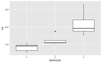
A convenient and well applicable visualization for comparing groups with respect to a metric variable is the boxplot. However, often, comparing means is accompanied by t-tests, ANOVAs, and friends. Such tests test the mean, not the median, and hence the boxplot is presenting the tested statistic. It would be better to align test and diagram. How can that be achieved using ggplot2? This posts demonstrates some possibilities.

First, let’s plot a boxplot.

Don’t forget to load the usual culprits.

library(tidyverse)
mtcars %>%
  ggplot +
  aes(x = factor(cyl), y = hp) +
  geom_boxplot() -> p1

p1

plot of chunk unnamed-chunk-2

Way one: Let ggplot compute the summary statistic

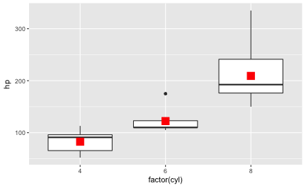
Now, let’s say we would like to add the mean for each group of cyl to the diagram. ggplot2 provides a function that will calculate summary statistics, such as the mean, for us: stat_summary. Let’s add this “layer” to the diagram:

p1 +
  stat_summary(fun.y = "mean", geom = "point", size = 5, color = "red", shape = 15)

plot of chunk unnamed-chunk-3

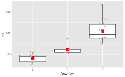
In addition to these two geoms (boxplot and ret dot for the mean), or as a replacement of one of these geoms, we may want to plot the raw data:

p1 +
  stat_summary(fun.y = "mean", geom = "point", size = 5, color = "red", shape = 15) +
  geom_jitter(color = "grey", width = .1)

plot of chunk unnamed-chunk-4

Way 2: Compute the summary statistic manually

One simple way to compute a summary statistic is this:

1. Take mtcars.
2. Group this dataframe by column "cyl".
3. Summarise the column "hp" by using the "mean" function (applies to each group as defined in step 2).
4. Save the result as a new dataframe.

The dplyr (tidyverse) code is a quite literal translation of this pseudo-syntax:

mtcars %>%
  group_by(cyl) %>%
  summarise(hp = mean(hp)) -> mtcars2
mtcars2
#> # A tibble: 3 x 2
#>     cyl        hp
#>   <dbl>     <dbl>
#> 1     4  82.63636
#> 2     6 122.28571
#> 3     8 209.21429

Now we can add a layer of points using this new dataframe (mtcars2):

mtcars %>%
  ggplot +
  aes(x = factor(cyl), y = hp) +
  geom_boxplot() +
  geom_point(data = mtcars2, color = "red", shape = 15, size = 5)

plot of chunk unnamed-chunk-6

Debrief

One may say, just don’t run a t-test, do a Wilcoxon, and everything is fine. Agreed. Some say that the t-test has more power than the Wilcoxon, but I personally don’t think that is much of an issue. However, my goal is not to judge about which test “is better”, but just to show some ways of plotting raw (detail) data alongside with a summary statistic.

Hadley Wickham has announced to depreceate dplyr::do in favor of purrr:map. In a recent post, I have made use of do, so some commentators informed me about that. In this post, I will show use cases of map, specifically as a replacement of do. map is for lists; read more about lists here.

library(tidyverse)
library(broom)

We will use mtcars as a sample dataframe (boring, I know, but convenient).

data(mtcars)

Cor is a function that takes a dataframe as its input

As in the last post, assume we would like to conduct a correlation test. First, let’s start simple using cor.

mtcars %>% 
  select_if(is.numeric) %>% 
  select(1:3) %>%   # to make it smaller
  cor
#>             mpg        cyl       disp
#> mpg   1.0000000 -0.8521620 -0.8475514
#> cyl  -0.8521620  1.0000000  0.9020329
#> disp -0.8475514  0.9020329  1.0000000

Here’s no need for purrr:map. map is essentially a looping device, taking a list as input. However, cor does not takes lists as input. It takes a whole dataframe (consisting of many lists). That’s even more practical than a looping function such as map.

cor.test via do and via map

Now let’s see where map makes sense. Consider cor.test from the last post. cor.test does not accept a dataframe as input, hence the dplyr logic does not apply well. Instead we have to build a workaround using do:

mtcars %>% 
  do(cor.test(.$hp, .$cyl) %>% tidy)
#>    estimate statistic      p.value parameter  conf.low conf.high
#> 1 0.8324475  8.228604 3.477861e-09        30 0.6816016 0.9154223
#>                                 method alternative
#> 1 Pearson's product-moment correlation   two.sided

Here we apply the function cor.test to two columns. Applying functions to columns (ie., lists) works smoothly with map and friends:

mtcars %>% 
  select(hp) %>%  # take out this line for iteration/loop
  map(~cor.test(.x, mtcars$cyl) %>% tidy)
#> $hp
#>    estimate statistic      p.value parameter  conf.low conf.high
#> 1 0.8324475  8.228604 3.477861e-09        30 0.6816016 0.9154223
#>                                 method alternative
#> 1 Pearson's product-moment correlation   two.sided

map applies a function to a list element

So, what does map do? It applies a function .fun over all elements of a list .list:

map(.list, .fun)

.list must either be a list or a simple vector. mapp is convenient for iteration as a replacement of “for-loops”:

mtcars %>% 
  select(hp, cyl, mpg) %>%  # only three for the sake of demonstration
  map(~cor.test(.x, mtcars$cyl) %>% tidy)
#> $hp
#>    estimate statistic      p.value parameter  conf.low conf.high
#> 1 0.8324475  8.228604 3.477861e-09        30 0.6816016 0.9154223
#>                                 method alternative
#> 1 Pearson's product-moment correlation   two.sided
#> 
#> $cyl
#>   estimate statistic p.value parameter conf.low conf.high
#> 1        1       Inf       0        30        1         1
#>                                 method alternative
#> 1 Pearson's product-moment correlation   two.sided
#> 
#> $mpg
#>    estimate statistic      p.value parameter   conf.low  conf.high
#> 1 -0.852162 -8.919699 6.112687e-10        30 -0.9257694 -0.7163171
#>                                 method alternative
#> 1 Pearson's product-moment correlation   two.sided

BTW, it would be nice to combine the tidy output elements ($hp, $cyl, $mpg) to a dataframe:

mtcars %>% 
  select(hp, cyl, mpg) %>%  # only three for the sake of demonstration
  map_df(~cor.test(.x, mtcars$cyl) %>% tidy)
#>     estimate statistic      p.value parameter   conf.low  conf.high
#> 1  0.8324475  8.228604 3.477861e-09        30  0.6816016  0.9154223
#> 2  1.0000000       Inf 0.000000e+00        30  1.0000000  1.0000000
#> 3 -0.8521620 -8.919699 6.112687e-10        30 -0.9257694 -0.7163171
#>                                 method alternative
#> 1 Pearson's product-moment correlation   two.sided
#> 2 Pearson's product-moment correlation   two.sided
#> 3 Pearson's product-moment correlation   two.sided

map_df maps the function (that’s what comes after “~”) to each list (ie., column) of mtcars. If possible, the resulting elements will be row-binded to a dataframe. To make the output of cor.test nice (ie., tidy) we again use tidy.

Extract elements from a list using map

Say, we are only interest in the p-value (OMG). How to extract each of the 3 p-values in our example?

mtcars %>% 
  select(hp, cyl, mpg) %>%  # only three for the sake of demonstration
  map(~cor.test(.x, mtcars$cyl) %>% tidy) %>% 
  map("p.value")
#> $hp
#> [1] 3.477861e-09
#> 
#> $cyl
#> [1] 0
#> 
#> $mpg
#> [1] 6.112687e-10

To extract several elements, say the p-value and r, we can use the [ operator:

mtcars %>% 
  select(hp, cyl, mpg) %>%  # only three for the sake of demonstration
  map(~cor.test(.x, mtcars$cyl) %>% tidy) %>% 
  map(`[`, c("p.value", "statistic"))
#> $hp
#>        p.value statistic
#> 1 3.477861e-09  8.228604
#> 
#> $cyl
#>   p.value statistic
#> 1       0       Inf
#> 
#> $mpg
#>        p.value statistic
#> 1 6.112687e-10 -8.919699

[ is some kind of “extractor” function; it extracts elements, and returns a list or data frame:

mtcars["hp"] %>% head
#>                    hp
#> Mazda RX4         110
#> Mazda RX4 Wag     110
#> Datsun 710         93
#> Hornet 4 Drive    110
#> Hornet Sportabout 175
#> Valiant           105
mtcars["hp"] %>% head %>% str
#> 'data.frame':	6 obs. of  1 variable:
#>  $ hp: num  110 110 93 110 175 105

x <- list(1, 2, 3)
x[1]
#> [[1]]
#> [1] 1

Maybe more convenient, there is a function called magrittr:extractor. It’s a wrapper aroung [:

library(magrittr)
mtcars %>% 
  select(hp, cyl, mpg) %>%  # only three for the sake of demonstration
  map(~cor.test(.x, mtcars$cyl) %>% tidy) %>% 
  map_df(extract, c("p.value", "statistic"))
#>        p.value statistic
#> 1 3.477861e-09  8.228604
#> 2 0.000000e+00       Inf
#> 3 6.112687e-10 -8.919699

Some say, the pipe (#tidyverse) makes analyses in R easier. I agree. This post demonstrates some examples.

Let’s take the mtcars dataset as an example.

data(mtcars)
?mtcars

Say, we would like to compute the correlation between gasoline consumption (mpg) and horsepower (hp).

Base approach 1

cor(mtcars[, c("mpg", "hp")])
##            mpg         hp
## mpg  1.0000000 -0.7761684
## hp  -0.7761684  1.0000000

We use the [-operator (function) to select the columns; note that df[, c(col1, col2)] sees dataframes as matrices, and spits out a dataframe, not a vector:

class(mtcars[, c("mpg", "hp")])
## [1] "data.frame"

That’s ok, because cor expects a matrix or a dataframe as input. Alternatively, we can understand dataframes as lists as in the following example.

Base approach 2

cor.test(x = mtcars[["mpg"]], y = mtcars[["hp"]])
##
## 	Pearson's product-moment correlation
##
## data:  mtcars[["mpg"]] and mtcars[["hp"]]
## t = -6.7424, df = 30, p-value = 1.788e-07
## alternative hypothesis: true correlation is not equal to 0
## 95 percent confidence interval:
##  -0.8852686 -0.5860994
## sample estimates:
##        cor
## -0.7761684

the [[-operator extracts a column from a list (a dataframe is technically a list), and extracts it as a vector. This is useful as some functions, such as cor.test don’t digest dataframes, but want vectors as input (here x, y).

Pipe approach 1

We will use dplyr for demonstrating the pipe approach.

library(dplyr)

mtcars %>%
  select(mpg, hp) %>%
  cor
##            mpg         hp
## mpg  1.0000000 -0.7761684
## hp  -0.7761684  1.0000000

If you are not acquainted with dplyr, the %>% operator can be translated as then do. More specifically, the result of the the lefthand side (lhs) is transferred as input to the righthand side (rhs).

Easy, right?

Pipe approach 2

We will need broom here, a package that renders some R output into a nice (ie, tidy) dataframe. For example, cor.test does not spit a nice dataframe when left in the wild. Applying tidy() from broom on the output, we will get a nice dataframe:

library(broom)

cor.test(x = mtcars[["mpg"]], y = mtcars[["hp"]]) %>% tidy
##     estimate statistic      p.value parameter   conf.low  conf.high
## 1 -0.7761684 -6.742389 1.787835e-07        30 -0.8852686 -0.5860994
##                                 method alternative
## 1 Pearson's product-moment correlation   two.sided
# same:
tidy(cor.test(x = mtcars[["mpg"]], y = mtcars[["hp"]]))
##     estimate statistic      p.value parameter   conf.low  conf.high
## 1 -0.7761684 -6.742389 1.787835e-07        30 -0.8852686 -0.5860994
##                                 method alternative
## 1 Pearson's product-moment correlation   two.sided

This code can be made simpler using dplyr:

mtcars %>%
  do(tidy(cor.test(.$mpg, .$hp)))
##     estimate statistic      p.value parameter   conf.low  conf.high
## 1 -0.7761684 -6.742389 1.787835e-07        30 -0.8852686 -0.5860994
##                                 method alternative
## 1 Pearson's product-moment correlation   two.sided

The function do from dplyr runs any function, provided it spits a dataframe. That’s why we first apply tidy from broom, and run do afterwards.

The . dot refers to the dataframe as handed over from the last step. We need this piece because cor.test does not know any variable by the name mpg (unless you have attached mtcars beforehands).

This code produces the same result:

mtcars %>%
  do(cor.test(.$mpg, .$hp) %>% tidy) %>%
  knitr::kable()
estimate statistic p.value parameter conf.low conf.high method alternative
-0.7761684 -6.742388 2e-07 30 -0.8852686 -0.5860994 Pearson’s product-moment correlation two.sided

Pipe appraoch 3

The package magrittr provides some pipe variants, most importantly perhaps the “exposition pipe”, %$%:

mtcars %$%
  cor.test(mpg, hp) %>%
  tidy
##     estimate statistic      p.value parameter   conf.low  conf.high
## 1 -0.7761684 -6.742389 1.787835e-07        30 -0.8852686 -0.5860994
##                                 method alternative
## 1 Pearson's product-moment correlation   two.sided

Why is it useful? Let’s spell out the code above in more detail.

  • Line 1: “Hey R, pick up mtcars but do not simply pass over this dataframe, but pull out each column and pass those columns over”
  • Line 2: “Run the function cor.test with hp and mpg” and then …
  • Line 3: “Tidy the result up. Not necessary here but quite nice”.

Remember that cor.test does not accept a dataframe as input. It expects two vectors. That’s why we need to transform the dataframe mtcars to a bundle of vectors (ie., the columns).

Recap

In sum, I think the pipe makes life easier. Of course, one needs to get used to it. But after a while, it’s much simpler than working with deeply nested [ brackets.

Enjoy the pipe!