Challenge 09 – Solution

Datum/Uhrzeit: 2026-01-09 22:41

“Eine Hackathon-Variante zur Evaluation der Klickdaten des KI-Tools ‘HaNS’”

Autor:in

Sebastian Sauer

Betrachten Sie dazu die Targets-Datei auf Github.

1 Setup

1.1 Libs

library(bench)
library(tidyverse)
library(data.table)
library(targets)
library(tictoc)
library(stringr)
library(tokenizers)

1.2 Other setup

source("_common.r")
list.files("funs", full.names = TRUE) |>
  purrr::walk(source)

options(digits = 3)
options(tinytable_tt_digits = 2)
Sys.setenv("VROOM_CONNECTION_SIZE" = 131072 * 4)

1.3 Load Targets

tar_load(c(
  data_files_list,
  data_all_fct,
  data_separated_filtered,
  course_and_uni_per_visit,
  n_action_type,
  time_spent_w_course_university
))

2 Musterlösung

2.1 Optimieren Sie Ihre Analyse-Pipeline

… (mit Blick auf alle Aufgaben des Hackathon) mit Blick auf Geschwindigkeit (des Durchlaufs der Pipeline). Berichten Sie die Laufzeit vor und nach der Optimierung. (ca. 3 Punkte mit jeweils 5 Sätzen)

2.1.1 CSV-Dateien schneller einlesen

2.1.1.1 Testdaten

d <- data_files_list[1:10]

2.1.1.2 Funktionen definieren

import_data1 <-
  function(d) {
  d |>
    map(~ read_csv(., show_col_types = FALSE)) |>
    rbindlist(fill = TRUE)
  }

import_data2 <-
  function(d) {
  rbindlist(
    lapply(d, fread, fill = TRUE, colClasses = "factor"),
    fill = TRUE
  )
  }


import_data3 <-
  function(d) {
  rbindlist(
    lapply(d, fread, fill = TRUE, colClasses = "character"),
    fill = TRUE
  )
}


import_data4 <- function(d) {
  rbindlist(
    lapply(d, fread, fill = TRUE, colClasses = "character", nThread = 4),
    fill = TRUE
  )
}


import_data4 <-
  function(d) {
  d |>
    map(~ data.table::fread(.x, fill = TRUE, colClasses = "factor", nThread = 4)) |>
    rbindlist(fill = TRUE)
  }

import_data5 <- function(d) {
  # Build shell command: concatenate all files
  cmd <- paste("cat", paste(shQuote(d), collapse = " "))

  # fread reads all files in one go (much faster than per-file lapply)
  DT <- fread(
    cmd = cmd,
    fill = TRUE,
    colClasses = "character",
    showProgress = FALSE
  )
}

2.1.1.3 Funktionen testen

test1 <- import_data1(d)
test2 <- import_data2(d)
test3 <- import_data3(d)
test4 <- import_data4(d)
test5 <- import_data5(d)

2.1.1.4 Effizienzvergleich

tic()
bm1 <- 
bench::mark(
  import_data1(d),
  import_data2(d),
  import_data3(d),
  import_data4(d),
  import_data5(d),
  check = FALSE,
  iterations = 1e1
)
toc()
## 61.169 sec elapsed

Ergebnisse im Überblick:

bm1 |> 
  dplyr::select(expression:n_gc) %>%
  knitr::kable(digits = 2)

expression	min	median	itr/sec	mem_alloc	gc/sec	n_itr	n_gc
import_data1(d)	1.52s	1.63s	0.60	23.82MB	2.63	10	44
import_data2(d)	983.36ms	1.06s	0.93	5.44MB	5.09	10	55
import_data3(d)	74.72ms	79.06ms	12.19	7.25MB	1.22	10	1
import_data4(d)	963.85ms	1.23s	0.84	5.44MB	4.94	10	59
import_data5(d)	50.46ms	52.57ms	18.56	4.82MB	0.00	10	0

Visualisierung:

## plot
plot_bm <- function(bm) {

bm$expression <- factor(bm$expression, levels = rev(bm$expression))
bench:::autoplot.bench_mark(bm, shape = 21, size = 2.5, color = "#333333aa") +
  ggplot2::aes(fill = expression) +
#  dataviz::theme_mwk() +
  ggplot2::theme(legend.position = "none",
    plot.caption = ggplot2::element_text(family = "Roboto Condensed")) +
  ggplot2::labs(x = NULL, y = "Time (mean task completion)")
}

plot_bm(bm1)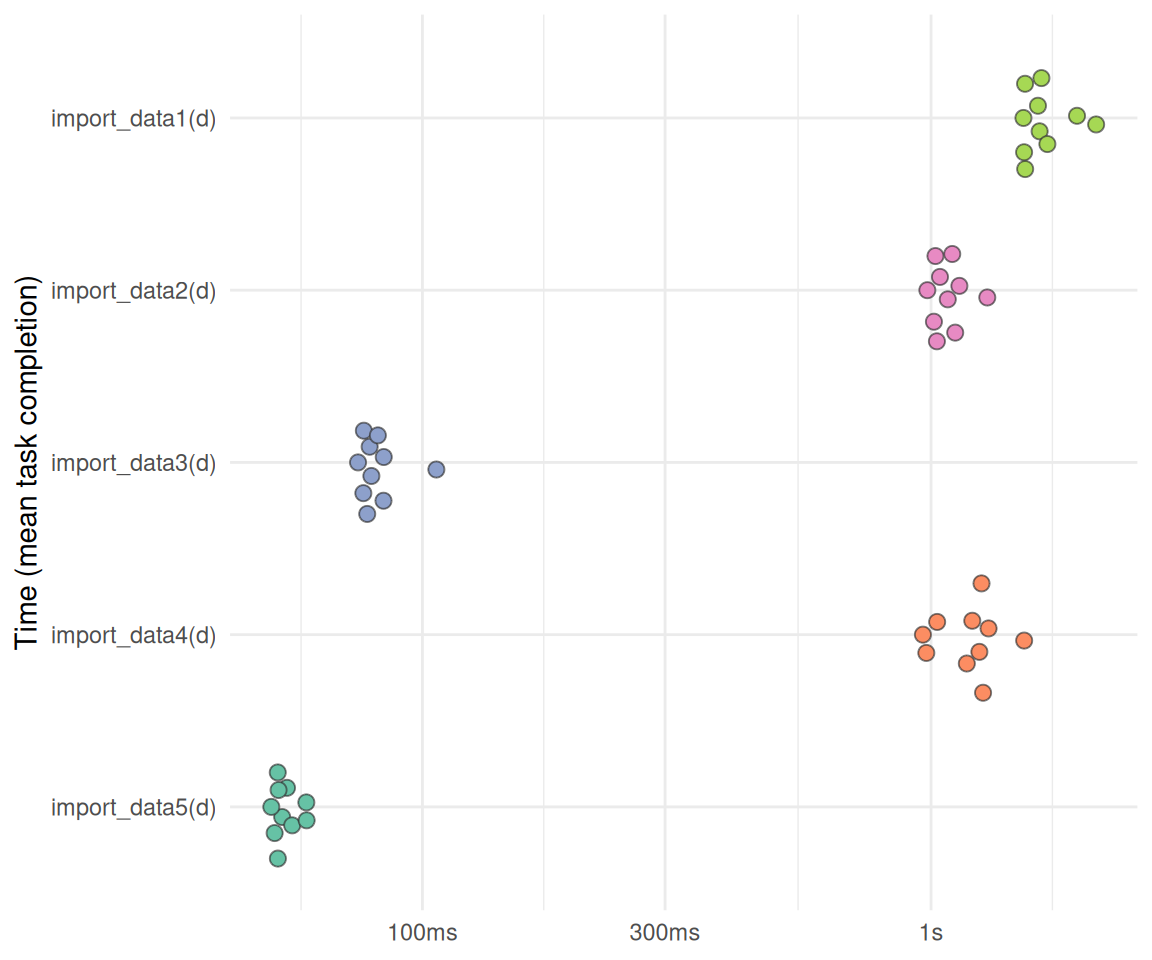

2.2 Daten schneller pivotieren

2.2.1 Testdaten

d_wide <- data_all_fct[, 1:1000]

2.2.2 Funktionen definieren

pivot1 <- function(d) {
  d |>
    select(idvisit, fingerprint, contains("actiondetails_")) |>
    mutate(across(everything(), as.character)) |>
    pivot_longer(-c(idvisit, fingerprint))
}


pivot2 <- function(d) {
  d_melt <- melt(
    as.data.table(d),
    id.vars = c("idvisit", "fingerprint"),
    measure.vars = patterns("actiondetails_"),
    variable.name = "action_count",
    value.name = "value"
  )
}


pivot3 <-  function(d) {
  vars_to_pivot <- grep("actiondetails_", names(d), value = TRUE)

  if (!is.data.table(d)) DT <- as.data.table(d) else DT <- d
  
  vars_idx <- grep("actiondetails_", names(DT)) 
  
  out <- melt(DT,
            id.vars = c("idvisit", "fingerprint"),
            measure.vars = vars_idx,
            variable.name = "variable",
            value.name = "value")
}

2.2.3 Funktionen testen

test_pivot1 <- pivot1(d_wide)
test_pivot2 <- pivot2(d_wide)
test_pivot3 <- pivot3(d_wide)

2.2.4 Effizienzvergleich

tic()
bm_pivot <- 
bench::mark(
 pivot1(d_wide),
 pivot2(d_wide),
 pivot3(d_wide),
 check = FALSE,
  iterations = 1e2
)
toc()
## 62.991 sec elapsed

Ergebnisse im Überblick:

bm_pivot |> 
  dplyr::select(expression:n_gc) %>%
  knitr::kable(digits = 2)

expression	min	median	itr/sec	mem_alloc	gc/sec	n_itr	n_gc
pivot1(d_wide)	330.8ms	402.1ms	2.46	159.3MB	1.94	56	44
pivot2(d_wide)	79.3ms	81.4ms	11.82	85.2MB	3.33	78	22
pivot3(d_wide)	73.9ms	74.8ms	12.88	71.7MB	2.45	84	16

plot_bm(bm_pivot)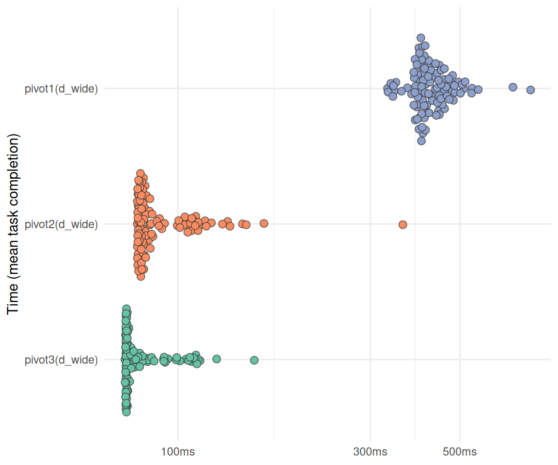

2.3 Daten schneller joinen

2.3.1 Testdaten

d_long <- data_separated_filtered 
d_date <- course_and_uni_per_visit

2.3.2 Funktionen definieren

join1 <- function(d_long, d_date) {
  setDT(d_long)
  setDT(d_date)
  setkey(d_date, "idvisit")

  # 1. Convert the factor column (x.idvisit) to an integer.
  # Factors store underlying values as integers, so we must first convert it to character
  # to avoid getting the factor level index, and then to integer.
  d_long[, idvisit := as.integer(as.character(idvisit))]
  d_date[, idvisit := as.integer(idvisit)]
  d_date[, fingerprint := NULL]

  # Join: [i, j]
  # DT[i] means join DT with i.
  # Left join syntax: A[B] where B is the "lookup" table (with the key set)

  # This performs the join:
  data_joined <- d_date[
    d_long,
    on = "idvisit"
  ]
}

join2 <- function(d_long, d_date) {
  
  d_date |> 
    mutate(idvisit = as.integer(as.character(idvisit))) |> 
    left_join(d_long)

}

2.3.3 Funktionen testen

d_join1 <- join1(d_long, d_date)
d_join2 <- join2(d_long, d_date)

2.3.4 Effizienzvergleich

bm_join <-
  mark(
    join1,
    join2,
    check = FALSE,
    iterations = 1e2
  )

plot_bm(bm_join)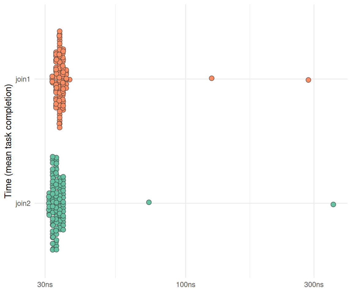

2.4 Optimieren Sie Ihre Analyse-Pipeline mit Blick auf Robustheit.

(ca. 3 Punkte mit jeweils 5 Sätzen)

2.4.1 Robusteres Pivotieren

pivot3_ribzst <-  function(d) {
  vars_to_pivot <- grep("actiondetails_", names(d), value = TRUE)

  if (!is.data.table(d)) DT <- as.data.table(d) else DT <- d
  
  ### Prüfen, ob benötigte Spalten vorhanden sind:
  # Check required id columns
  required_ids <- c("idvisit", "fingerprint")
  missing_ids <- setdiff(required_ids, names(DT))
  if (length(missing_ids) > 0) {
    stop("Missing required id columns: ", paste(missing_ids, collapse = ", "))
  }
  
  
  vars_idx <- grep("actiondetails_", names(DT)) 
  
  out <- melt(DT,
            id.vars = c("idvisit", "fingerprint"),
            measure.vars = vars_idx,
            variable.name = "variable",
            value.name = "value")
}

2.4.2 Robusteres Importieren

import_data5 <- function(d) {
  # Build shell command: concatenate all files
  cmd <- paste("cat", paste(shQuote(d), collapse = " "))

  # fread reads all files in one go (much faster than per-file lapply)
  DT <- fread(
    cmd = cmd,
    fill = TRUE,
    colClasses = "character",
    showProgress = FALSE
  )
}

import_data5_robust <- function(d) {
  
  # Check input
  if (length(d) == 0) {
    warning("No files provided. Returning empty data.table.")
    return(data.table())
  }
  
  # Check: Ensure all files exist
  missing_files <- d[!file.exists(d)]
  if (length(missing_files) > 0) {
    stop("The following files do not exist: ", paste(missing_files, collapse = ", "))
  }
  
  # Build safe shell command
  cmd <- paste("cat", paste(shQuote(d), collapse = " "))
  
  # fread reads all files in one go
  DT <- fread(
    cmd = cmd,
    fill = TRUE,
    colClasses = "character",
    showProgress = FALSE
  )
  

  # Check: Warn if column counts vary across files (optional)
  if (length(unique(ncol(DT))) > 1) {
    warning("Column counts vary across files. Some columns may have been filled with NA.")
  }
  
  # Explicitly Return the data.table
  return(DT)
}

2.4.3 Robusteres Berechnen der Promptlänge

Ursprüngliche Funktion:

compute_prompt_length <- function(data, no_prompt_text = TRUE) {
  #' Compute the length of a prompt in characters
  #' This function computes the length of a given prompt in terms of number of characters.
  #' It takes a single argument 'prompt', which is expected to be a string.

  # if (!is.character(data$value)) {
    # stop("Input must be a character string.")
  # }

  llm_interactions <-
    data |> 
    select(type, value, idvisit) |> 
    filter(type == "subtitle") |> 
    mutate(value = as.character(value)) |>
    filter(str_detect(value, "message_to_llm"))

  prompts <-
    llm_interactions |>
    mutate(prompt = str_extract(value, '(?<=Action: \\"\").*?(?=\\"\\")')) |>
    mutate(token_length = lengths(tokenize_words(prompt))) 
  

  if (no_prompt_text) {
    prompts <- prompts |> select(-prompt)
  }

  return(prompts)
}

# str_match(txt, '""([^"]+)""')
# txt

Robustere Version:

compute_prompt_length_robust <- function(data, no_prompt_text = TRUE) {
  
  # Input validation:
  if (!is.data.frame(data)) {
    stop("Input 'data' must be a data.frame or tibble.")
  }
  
  # Check required cols:
  required_cols <- c("type", "value", "idvisit")
  missing_cols <- setdiff(required_cols, names(data))
  if (length(missing_cols) > 0) {
    stop("Missing required columns: ", paste(missing_cols, collapse = ", "))
  }
  
  # Filter only subtitle rows with "message_to_llm"
  llm_interactions <- data %>%
    select(all_of(required_cols)) %>%
    filter(type == "subtitle") %>%
    mutate(value = as.character(value)) %>%
    filter(str_detect(value, "message_to_llm"))
  
  if (nrow(llm_interactions) == 0) {
    warning("No subtitle rows containing 'message_to_llm' found.")
    return(tibble::tibble())
  }
  
  # Extract prompt safely
  prompts <- llm_interactions %>%
    mutate(
      prompt = str_extract(value, '(?<=Action: \\"\").*?(?=\\"\\")')
    )
  
  # Compute token length, handling NA prompts:
  prompts <- prompts %>%
    mutate(
      token_length = ifelse(
        is.na(prompt) | prompt == "",
        0L,
        lengths(tokenize_words(prompt))
      )
    )
  
  # Optionally remove the prompt column
  if (no_prompt_text && "prompt" %in% names(prompts)) {
    prompts <- prompts %>% select(-prompt)
  }
  
  prompts
}

2.5 Optimieren Sie Ihre Analyse-Pipeline mit Blick auf Allgemeinheit und Flexibilität

2.5.1 Explizites `return`-Statement

Am Ende einer Funktion kann man explizit schreiben, welches Objekt die Funktion zurückgibt:


import_data5_with_return <- function(d) {
  # Build shell command: concatenate all files
  cmd <- paste("cat", paste(shQuote(d), collapse = " "))

  # fread reads all files in one go (much faster than per-file lapply)
  DT <- fread(
    cmd = cmd,
    fill = TRUE,
    colClasses = "character",
    showProgress = FALSE
  )
  # Achtung, mit return:
  return(DT)
}

2.5.2 `idvisit` vs. `id_visit`

Tja, hat meine ID-Variable jetzt einen Unterstrich oder nicht?

Ist doch egal, unser Code akzeptiert beide Varianten!

d1 <- tibble(idvisit = c(1,2,3),
             var = c("a", "b", "c"),
             value = c(10, 20, 30))

d2 <- tibble(id_visit = c(1,2,3),
             var = c("a", "b", "c"),
             value = c(10, 20, 30))

idvar <- c("id_visit", "idvisit") 

d1 |> select(any_of(idvar))

idvisit
1
2
3

d2 |> select(any_of(idvar))

id_visit
1
2
3

Vielleicht noch besser: An einer Stelle in der Pipeline (eher zu Beginn) den Namen auf einen Standard bringen, z.B. idvisit.

2.5.3 Funktionen nicht hart-verdrahten

Ursprüngliche Funktion:

add_dates_to_n_action_type <- function(data, data_time) {

  data_time$idvisit <- as.integer(data_time$idvisit)

  n_action_type_per_month <-
    data |>
    select(nr, idvisit, category) |>
    ungroup() |>
    left_join(data_time) 
    #select(-c(dow, hour, nr)) |>
    #drop_na() |>
    #mutate(month_start = floor_date(date_time, "month")) |>
    #count(month_start, category)
}

Allgemeinere Funktion:

add_dates_to_n_action_type_more_general <- function(data, data_time, idvar = "idvisit") {

  # Convert join variable to integer in both data frames
  data[[idvar]] <- as.integer(data[[idvar]])
  data_time[[idvar]] <- as.integer(as.character(data_time[[idvar]]))

  n_action_type_per_month <- data |>
    select(nr, all_of(idvar), category) |>
    left_join(data_time, by = idvar)

  return(n_action_type_per_month)
}

Test:

d_not_so_general <- add_dates_to_n_action_type(
    data = n_action_type,
    data_time = time_spent_w_course_university)

d_more_general <- add_dates_to_n_action_type_more_general(
  data = n_action_type, 
  data_time = time_spent_w_course_university)


identical(d_not_so_general, d_more_general)
## [1] TRUE

2.5.4 Rechtecke, um Semester und Ferien optisch zu unterscheiden

"funs/comp_semester_rects.R"
## [1] "funs/comp_semester_rects.R"

2.5.5 Frage die KI

Alle Funktionen in eine KI hochladen und nach Optimierungspotenzial fragen.

Z.B. in “Google Notebook LM” muss man die R-Dateien vorher in Txt-Dateien umwandeln: rename 's/\.R$/.txt/' *.R

2.6 Diskutieren Sie Pro und Contra der Versionierungssoftware git.

Git: git push origin master.

2.7 Diskutieren Sie Pro und Contra der Notizen-Software Obsidian.

Video von No Boilerplate und [Folien]/https://www.namtao.com/obsidian-for-learning/

2.7.1 Pro

Plain text
Markdown
Lokale Dateien
E2EE
Tags, Links
Open source
Viele Plugins
offline und online
alle Plattformen
schnell
kein Lock-in

2.8 Contra

Nicht so gut für gemeinsames Arbeiten

2.9 Erläutern Sie Ihre Datensicherheit und Backup-Strategie während des Projekts. Wie schützen Sie sich vor Datenverlust?

2.9.1 Backup

Github
Lokale Backups

2.9.2 Datensicherheit

Cryptomator
KeepassXC

2.10 Life Hacks

Nicht zu spät anfangen :-)
Schreibtisch frei räumen
Lange Zeitblöcke einplanen
Obsidian für Notizen
Wochenende frei halten
Den Sinn sehen

2.11 Text-Editoren

RStudio
Positron (Outline feature is broken)
VIM
NeoVIM

2.12 Ohne R

Python
Positron
Jupyter Notebooks

2.13 sessionInfo

sessioninfo::session_info()
## ─ Session info ───────────────────────────────────────────────────────────────
##  setting  value
##  version  R version 4.5.1 (2025-06-13)
##  os       Ubuntu 25.10
##  system   x86_64, linux-gnu
##  ui       X11
##  language (EN)
##  collate  de_DE.UTF-8
##  ctype    de_DE.UTF-8
##  tz       Europe/Berlin
##  date     2026-01-09
##  pandoc   3.6.3 @ /usr/lib/rstudio/resources/app/bin/quarto/bin/tools/x86_64/ (via rmarkdown)
##  quarto   1.8.25 @ /usr/lib/rstudio/resources/app/bin/quarto/bin/quarto
## 
## ─ Packages ───────────────────────────────────────────────────────────────────
##  package      * version date (UTC) lib source
##  backports      1.5.0   2024-05-23 [3] CRAN (R 4.4.1)
##  base64url      1.4     2018-05-14 [3] CRAN (R 4.0.1)
##  beeswarm       0.4.0   2021-06-01 [3] CRAN (R 4.1.1)
##  bench        * 1.1.4   2025-01-16 [3] CRAN (R 4.4.3)
##  bit            4.6.0   2025-03-06 [3] CRAN (R 4.4.3)
##  bit64          4.6.0-1 2025-01-16 [3] CRAN (R 4.5.0)
##  callr          3.7.6   2024-03-25 [3] CRAN (R 4.4.0)
##  cli            3.6.5   2025-04-23 [1] CRAN (R 4.5.1)
##  codetools      0.2-20  2024-03-31 [4] CRAN (R 4.3.3)
##  crayon         1.5.3   2024-06-20 [3] CRAN (R 4.4.2)
##  data.table   * 1.17.8  2025-07-10 [1] RSPM (R 4.5.1)
##  dichromat      2.0-0.1 2022-05-02 [3] CRAN (R 4.2.0)
##  digest         0.6.39  2025-11-19 [1] CRAN (R 4.5.1)
##  dplyr        * 1.1.4   2023-11-17 [3] CRAN (R 4.4.2)
##  evaluate       1.0.5   2025-08-27 [1] CRAN (R 4.5.1)
##  farver         2.1.2   2024-05-13 [3] CRAN (R 4.4.1)
##  fastmap        1.2.0   2024-05-15 [3] CRAN (R 4.4.1)
##  forcats      * 1.0.0   2023-01-29 [3] CRAN (R 4.2.2)
##  generics       0.1.4   2025-05-09 [1] CRAN (R 4.5.1)
##  ggbeeswarm     0.7.2   2023-04-29 [3] CRAN (R 4.3.1)
##  ggplot2      * 4.0.1   2025-11-14 [1] RSPM (R 4.5.1)
##  glue           1.8.0   2024-09-30 [3] CRAN (R 4.4.2)
##  gtable         0.3.6   2024-10-25 [3] CRAN (R 4.4.2)
##  hms            1.1.3   2023-03-21 [3] CRAN (R 4.3.1)
##  htmltools      0.5.8.1 2024-04-04 [3] CRAN (R 4.4.0)
##  htmlwidgets    1.6.4   2023-12-06 [3] CRAN (R 4.3.2)
##  igraph         2.1.4   2025-01-23 [3] CRAN (R 4.5.0)
##  jsonlite       2.0.0   2025-03-27 [1] CRAN (R 4.5.1)
##  knitr          1.50    2025-03-16 [3] CRAN (R 4.4.3)
##  lifecycle      1.0.4   2023-11-07 [3] CRAN (R 4.3.2)
##  lubridate    * 1.9.4   2024-12-08 [3] CRAN (R 4.4.2)
##  magrittr       2.0.4   2025-09-12 [1] CRAN (R 4.5.1)
##  pillar         1.11.1  2025-09-17 [1] CRAN (R 4.5.1)
##  pkgconfig      2.0.3   2019-09-22 [3] CRAN (R 4.0.1)
##  prettyunits    1.2.0   2023-09-24 [3] CRAN (R 4.3.1)
##  processx       3.8.6   2025-02-21 [3] CRAN (R 4.4.3)
##  profmem        0.6.0   2020-12-13 [3] CRAN (R 4.0.3)
##  ps             1.9.0   2025-02-18 [3] CRAN (R 4.4.3)
##  purrr        * 1.2.0   2025-11-04 [1] RSPM (R 4.5.1)
##  R6             2.6.1   2025-02-15 [3] CRAN (R 4.4.3)
##  RColorBrewer   1.1-3   2022-04-03 [3] CRAN (R 4.2.0)
##  Rcpp           1.1.0   2025-07-02 [3] CRAN (R 4.5.1)
##  readr        * 2.1.6   2025-11-14 [1] RSPM
##  rlang          1.1.6   2025-04-11 [1] CRAN (R 4.5.1)
##  rmarkdown      2.30    2025-09-28 [1] RSPM (R 4.5.1)
##  rstudioapi     0.17.1  2024-10-22 [3] CRAN (R 4.4.1)
##  S7             0.2.1   2025-11-14 [1] RSPM (R 4.5.1)
##  scales         1.4.0   2025-04-24 [1] RSPM (R 4.5.1)
##  secretbase     1.0.5   2025-03-04 [1] RSPM
##  sessioninfo    1.2.3   2025-02-05 [3] CRAN (R 4.4.3)
##  SnowballC      0.7.1   2023-04-25 [1] RSPM
##  stringi        1.8.7   2025-03-27 [1] CRAN (R 4.5.1)
##  stringr      * 1.6.0   2025-11-04 [1] CRAN (R 4.5.1)
##  targets      * 1.11.4  2025-09-13 [1] RSPM
##  tibble       * 3.3.0   2025-06-08 [1] CRAN (R 4.5.1)
##  tictoc       * 1.2.1   2024-03-18 [1] RSPM
##  tidyr        * 1.3.1   2024-01-24 [3] CRAN (R 4.3.2)
##  tidyselect     1.2.1   2024-03-11 [3] CRAN (R 4.4.0)
##  tidyverse    * 2.0.0   2023-02-22 [3] CRAN (R 4.4.2)
##  timechange     0.3.0   2024-01-18 [3] CRAN (R 4.4.3)
##  tokenizers   * 0.3.0   2022-12-22 [1] RSPM
##  tzdb           0.5.0   2025-03-15 [3] CRAN (R 4.4.3)
##  vctrs          0.6.5   2023-12-01 [3] CRAN (R 4.3.2)
##  vipor          0.4.7   2023-12-18 [3] CRAN (R 4.3.2)
##  vroom          1.6.5   2023-12-05 [3] CRAN (R 4.3.2)
##  withr          3.0.2   2024-10-28 [3] CRAN (R 4.4.1)
##  xfun           0.54    2025-10-30 [1] CRAN (R 4.5.1)
##  yaml           2.3.10  2024-07-26 [3] CRAN (R 4.4.1)
## 
##  [1] /home/sebastian-sauer/R/x86_64-pc-linux-gnu-library/4.5
##  [2] /usr/local/lib/R/site-library
##  [3] /usr/lib/R/site-library
##  [4] /usr/lib/R/library
##  * ── Packages attached to the search path.
## 
## ──────────────────────────────────────────────────────────────────────────────

Wiederverwendung

MIT

Zitat

Mit BibTeX zitieren:

@online{sauer,
  author = {Sauer, Sebastian},
  title = {Challenge 09 -\/- Solution},
  url = {https://sebastiansauer.github.io/hans-hackathon2025/challenge09-solution.html},
  langid = {de-DE}
}

Bitte zitieren Sie diese Arbeit als:

Sauer, Sebastian. n.d. “Challenge 09 -- Solution.” https://sebastiansauer.github.io/hans-hackathon2025/challenge09-solution.html.