Challenge 07 – Solution

Datum/Uhrzeit: 2026-01-09 15:24

“Eine Hackathon-Variante zur Evaluation der Klickdaten des KI-Tools ‘HaNS’”

Autor:in

Sebastian Sauer

Betrachten Sie dazu die Targets-Datei auf Github.

1 Setup

1.1 Libs

1.2 Other setup

source("_common.r")
list.files("funs", full.names = TRUE) |>
  purrr::walk(source)

options(digits = 3)
options(tinytable_tt_digits = 2)

1.3 Load Targets

tar_load(c(
 data_separated_filtered,
 data_separated_filtered_date_uni_course,
 idvisit_has_llm,
 prompt_length,
 prompt_length_date_uni_course,
 n_interactions_w_llm_course_date_course_uni,
 llm_response_text,
 llm_response_text_date_course_uni
))

2 Musterlösung

2.1 Auf welche Art und wie oft wird mit dem LLM interagiert? Suchen Sie dafür nach eventcategory “llm” – zählen Sie die Werte der verschiedenen Kategorien.

data_separated_filtered_ai <-
  data_separated_filtered |>
  filter(type == "eventcategory") |>
  filter(str_detect(value, "llm")) |>
  count(value, sort = TRUE) |>
  mutate(prop = n / sum(n))

data_separated_filtered_ai |> 
  kable(digits = 1)

value	n	prop
message_to_llm	166	0.3
message_to_llm_de	162	0.3
llm_response_de	140	0.2
select_transcript_text_for_llm_context	108	0.2
clear_transcript_text_for_llm_context	3	0.0
llm_response_en	1	0.0
message_to_llm_en	1	0.0

Als “Bild-Tabelle”:

data_separated_filtered_ai |>
  mutate(prop = round(prop, 3)) |>
  ggtexttable()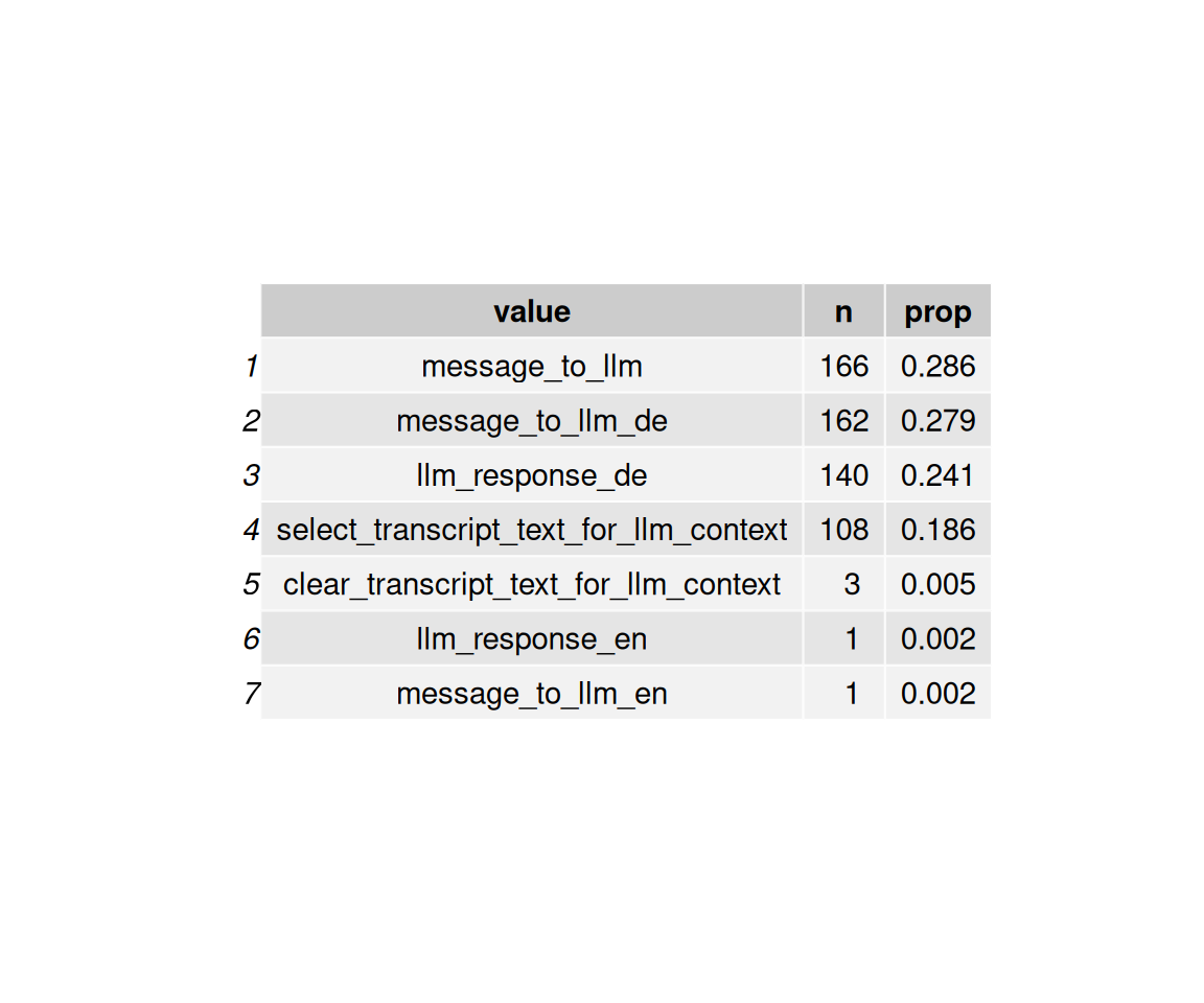

Man beachte das Sortieren der Balken:

data_separated_filtered_ai |> 
  ggplot() +
  aes(x = prop, y = value) +
  geom_col()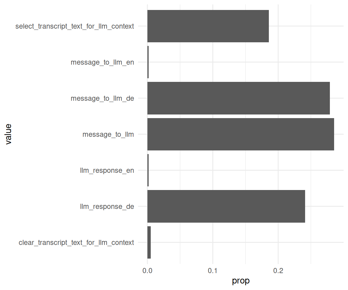

data_separated_filtered_ai |> 
  mutate(value = fct_reorder(.f = value, .x = prop)) |> 
  ggplot() +
  aes(x = prop, y = value) +
  geom_col()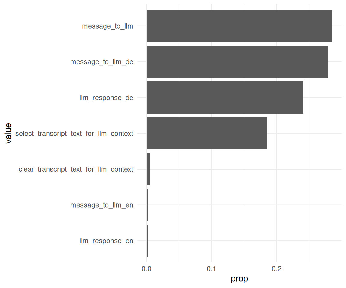

2.2 Wie viele Nachrichten werden an das LLM gesendet von den Besuchern?

llm_interactions <-
  data_separated_filtered |>
  filter(str_detect(value, "message_to_llm"))

Statistiken:

llm_interactions_count <-
  llm_interactions |>
  count(idvisit, sort = TRUE) |>
  rename(messages_to_llm_n = n)

llm_interactions_count |>
  describe_distribution(messages_to_llm_n, centrality = c("mean", "median")) |>
  print_md()

Variable	Median	MAD	Mean	SD	IQR	Range	Skewness	Kurtosis	n	n_Missing
messages_to_llm_n	4	1.48	9.40	8.88	8	(2.00, 44.00)	2.31	5.62	70	0

Man beachte das print_md.

gghistogram(
  llm_interactions_count,
  x = "Number of messages sent to the LLM",
  y = "Count",
  bins = 10,
  add = "median"
) +
  labs(caption = "The vertical dotted line denotes the median.")
## Error in `purrr::pmap()`:
## ℹ In index: 1.
## ℹ With name: Count.
## Caused by error in `ans[npos] <- rep(no, length.out = len)[npos]`:
## ! Ersetzung hat Länge 0

2.3 Wie groß ist der Anteil der Besucher, die mit dem LLM interagieren?

Für Tabellen gibt es mehrere Möglichkeiten, z.B. kable oder gt.

data_separated_filtered_llm_interact <-
  data_separated_filtered |>
  mutate(has_llm = str_detect(value, "llm")) |>
  group_by(idvisit) |>
  summarise(llm_used_during_visit = any(has_llm == TRUE)) |>
  count(llm_used_during_visit) |>
  mutate(prop = round(n / sum(n), 2))

data_separated_filtered_llm_interact |>
  gt()

llm_used_during_visit	n	prop
FALSE	2644	0.94
TRUE	180	0.06

Bonus - Auswertung pro fingerprint:

data_separated_filtered_llm_interact_fingerprint <-
  data_separated_filtered |>
  mutate(has_llm = str_detect(value, "llm")) |>
  group_by(fingerprint) |>
  summarise(llm_used_during_visit = any(has_llm == TRUE)) |>
  count(llm_used_during_visit) |>
  mutate(prop = round(n / sum(n), 2))

data_separated_filtered_llm_interact_fingerprint |>
  gt()

llm_used_during_visit	n	prop
FALSE	1158	0.91
TRUE	121	0.09

2.4 Wie groß ist der Anteil der Besucher, die mit dem LLM interagieren, pro Kunde (Hochschule)?

data_separated_filtered_llm_interact_uni <- 
data_separated_filtered_date_uni_course |> 
  mutate(has_llm = str_detect(value, "llm")) |>
  group_by(university, idvisit) |>
  summarise(llm_used_during_visit = any(has_llm == TRUE)) |>
  count(llm_used_during_visit) |>
  mutate(prop = round(n / sum(n), 2))

2.4.1 Mit `gt`

data_separated_filtered_llm_interact_uni |> 
  gt()

llm_used_during_visit	n	prop
evhn
FALSE	1	0.25
TRUE	3	0.75
hnu
FALSE	8	0.89
TRUE	1	0.11
hswt
FALSE	816	0.97
TRUE	29	0.03
th-nuernberg
FALSE	779	0.92
TRUE	71	0.08
th-owl
FALSE	1	1.00
thi
FALSE	1	1.00
NA
FALSE	1038	0.93
TRUE	76	0.07

2.4.2 Mit `kable`

data_separated_filtered_llm_interact_uni |> 
  kable()

university	llm_used_during_visit	n	prop
evhn	FALSE	1	0.25
evhn	TRUE	3	0.75
hnu	FALSE	8	0.89
hnu	TRUE	1	0.11
hswt	FALSE	816	0.97
hswt	TRUE	29	0.03
th-nuernberg	FALSE	779	0.92
th-nuernberg	TRUE	71	0.08
th-owl	FALSE	1	1.00
thi	FALSE	1	1.00
NA	FALSE	1038	0.93
NA	TRUE	76	0.07

2.4.3 Mit `tinytable`

data_separated_filtered_llm_interact_uni |> 
  tt()

university	llm_used_during_visit	n	prop
evhn	FALSE	1	0.25
evhn	TRUE	3	0.75
hnu	FALSE	8	0.89
hnu	TRUE	1	0.11
hswt	FALSE	816	0.97
hswt	TRUE	29	0.03
th-nuernberg	FALSE	779	0.92
th-nuernberg	TRUE	71	0.08
th-owl	FALSE	1	1.00
thi	FALSE	1	1.00
NA	FALSE	1038	0.93
NA	TRUE	76	0.07

2.5 Verändert sich der Anteil der Besucher, die mit dem LLM interagieren, im Zeitverlauf?

idvisit_has_llm_timeline <-
  idvisit_has_llm |>
  count(year_month, uses_llm) |>
  ungroup() |>
  group_by(year_month) |>
  mutate(prop = round(n / sum(n), 2))

idvisit_has_llm_timeline

idvisit_has_llm |>
  count(year_month, uses_llm) |>
  ungroup() |>
  mutate(year_month_date = ymd(paste0(year_month, "-01"))) |>
  group_by(year_month_date) |>
  mutate(prop = n / sum(n)) |>
  ggplot(aes(
    x = year_month_date,
    y = prop,
    color = uses_llm,
    groups = uses_llm
  )) +
  # --- Highlight March–July (approx 1 Mar to 31 Jul) ---
  annotate(
    "rect",
    xmin = as.Date("2023-03-01"),
    xmax = as.Date("2023-07-31"),
    ymin = -Inf,
    ymax = Inf,
    alpha = 0.2,
    fill = "skyblue"
  ) +

  annotate(
    "rect",
    xmin = as.Date("2024-03-01"),
    xmax = as.Date("2024-07-31"),
    ymin = -Inf,
    ymax = Inf,
    alpha = 0.2,
    fill = "skyblue"
  ) +
  annotate(
    "rect",
    xmin = as.Date("2025-03-01"),
    xmax = as.Date("2025-07-31"),
    ymin = -Inf,
    ymax = Inf,
    alpha = 0.2,
    fill = "skyblue"
  ) +

  # --- Highlight October–February (semester break or 2nd term) ---
  annotate(
    "rect",
    xmin = as.Date("2023-10-01"),
    xmax = as.Date("2024-02-28"),
    ymin = -Inf,
    ymax = Inf,
    alpha = 0.2,
    fill = "orange"
  ) +
  # annotate("rect",
  #          xmin = as.Date("2024-10-01"), xmax = as.Date("2024-02-28"),
  #          ymin = -Inf, ymax = Inf, alpha = 0.2, fill = "orange") +
  annotate(
    "rect",
    xmin = as.Date("2024-10-01"),
    xmax = as.Date("2025-02-28"),
    ymin = -Inf,
    ymax = Inf,
    alpha = 0.2,
    fill = "orange"
  ) +
  geom_point() +
  geom_line(aes(group = uses_llm)) +
  labs(
    title = "Visitors, die mit dem LLM interagieren im Zeitverlauf (Anteile)"
  ) +
  scale_x_date(breaks = pretty_breaks())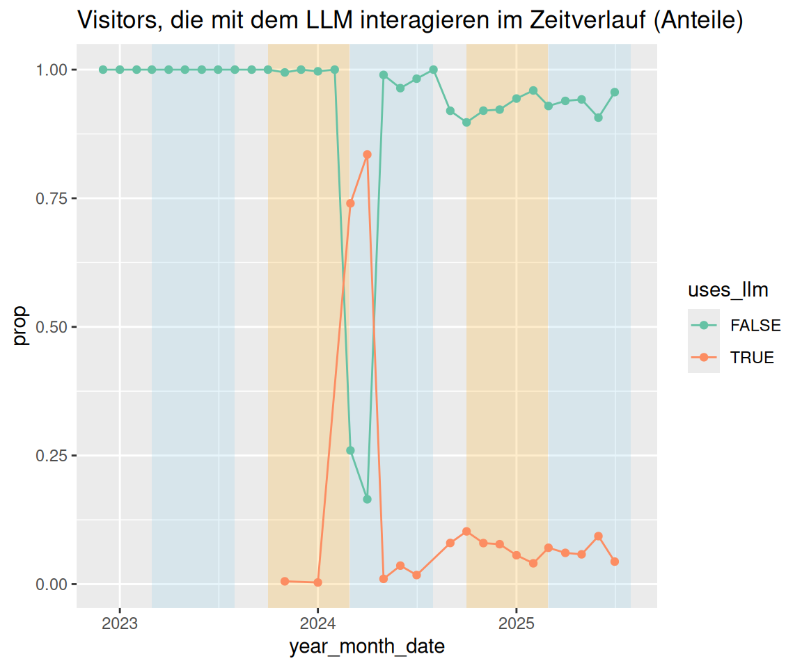

pretty_breaks sind eine praktische Angelegenheit.

idvisit_has_llm |>
  count(year_month, uses_llm) |>
  ungroup() |>
  mutate(year_month_date = ymd(paste0(year_month, "-01"))) |>
  group_by(year_month_date) |>
  # ADDED: Calculate the proportion
  mutate(proportion = n / sum(n)) |>

  # Plot using the new 'proportion' variable
  ggplot(aes(x = year_month_date, y = proportion, fill = uses_llm)) +

  # ADDED: Use position = "fill"
  geom_area(position = "fill") +

  # ADDED: Format y-axis as percentage
  scale_y_continuous(labels = scales::label_percent()) +

  labs(
    title = "Anteil der Besucher, die mit dem LLM interagieren (Prozent)",
    y = "Prozentualer Anteil der Besucher",
    fill = "Interagiert mit LLM",
    x = "Datum"
  ) +
  scale_x_date(breaks = pretty_breaks())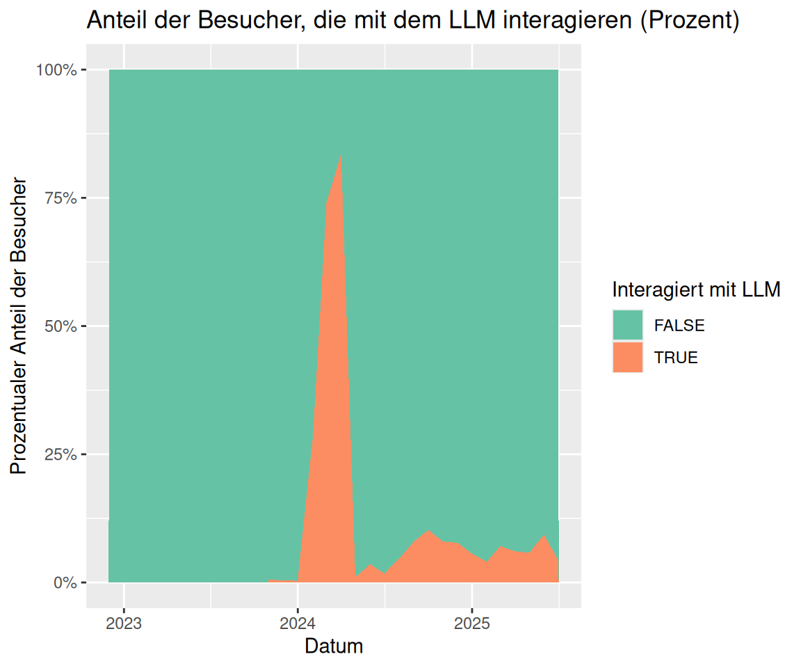

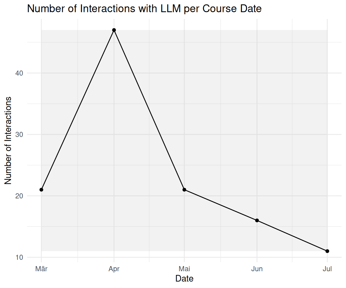
2.6 Bonus: Veränderung der LLM-Nutzung im Zeitverlauf

# --- 1. Prepare Data ---
# Your original data processing for the plot
plot_data <- n_interactions_w_llm_course_date_course_uni |>
  group_by(floor_date_month) |>
  summarise(n = n()) |>
  ungroup() # Ungroup after summarise for easier use with ggplot

# --- 2. Determine Plot Range for Rectangles ---
# Find the min/max year and n-count from your *processed* plot_data
min_date <- min(plot_data$floor_date_month, na.rm = TRUE)
max_date <- max(plot_data$floor_date_month, na.rm = TRUE)
min_year <- year(min_date)
max_year <- year(max_date)

# Determine the Y-axis bounds for the rectangles
y_min <- min(plot_data$n, na.rm = TRUE)
y_max <- max(plot_data$n, na.rm = TRUE)

# --- 3. Calculate the Rectangle Coordinates (rect_data) ---

# Generate years for the rectangles, ensuring we cover the full range
# including potentially starting a "winter" semester in the min_year-1
# and ending in max_year+1
rect_years <- seq(min_year - 1, max_year + 1)

# Summer semester: March 1 (Y) to July 1 (Y)
summer_rects <- tibble(year = rect_years) |>
  mutate(
    xmin = ymd(paste0(year, "-03-01")),
    xmax = ymd(paste0(year, "-07-01"))
  )

# Winter semester: October 1 (Y) to February 1 (Y+1)
winter_rects <- tibble(year = rect_years) |>
  mutate(
    xmin = ymd(paste0(year, "-10-01")),
    xmax = ymd(paste0(year + 1, "-02-01"))
  )

# Combine, set Y bounds, and filter to the actual plot area
rect_data <- bind_rows(summer_rects, winter_rects) |>
  mutate(ymin = y_min, ymax = y_max) |>
  # Only keep rectangles that are fully or partially within the plot's X range
  filter(
    xmin <= max_date,
    xmax >= min_date
  )

# --- 4. Generate the Final Plot ---
plot_data |>
  ggplot(aes(x = floor_date_month, y = n)) +
  # Add the transparent grey rectangles first
  geom_rect(
    data = rect_data,
    aes(xmin = xmin, xmax = xmax, ymin = ymin, ymax = ymax),
    fill = "grey",
    alpha = 0.2,
    inherit.aes = FALSE # Essential to use the rect_data columns
  ) +
  # Then plot the lines and points on top
  geom_line() +
  geom_point() + # Added point layer for clarity at each month
  theme_minimal() +
  labs(
    title = "Number of Interactions with LLM per Course Date",
    x = "Date",
    y = "Number of Interactions"
  )

2.7 Die Länge der Prompts an das LLM ist wichtig zu wissen (da potenziell teuer). Werten Sie die Länge der Prompts an das LLM pro Visit aus. Messen Sie die Länge der Prompts in Tokens.

prompt_length_no_prompts <-
  prompt_length |>
  select(-any_of(c("prompt", "value", "type")))

prompt_length_no_prompts |>
  describe_distribution(token_length) |>
  print_md()

Variable	Mean	SD	IQR	Range	Skewness	Kurtosis	n	n_Missing
token_length	6.77	4.47	4.50	(1.00, 26.00)	1.30	2.39	329	0

prompt_length_no_prompts |>
  ggplot(aes(x = token_length)) +
  geom_histogram(binwidth = 5) +
  labs(
    title = "Length of prompts sent to the LLM",
    x = "Prompt length (in tokens)",
    y = "Number of prompts"
  ) +
  theme_minimal()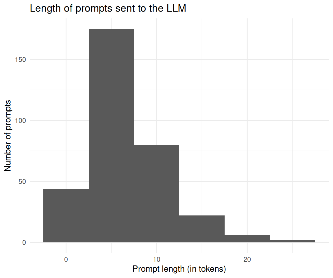

2.8 Unterscheidet sich die Token-Länge zwischen den Kunden (d.h. Hochschulen)?

prompt_length_date_uni_course |>
  group_by(university) |>
  describe_distribution(token_length) |>
  print_md()

university	Variable	Mean	SD	IQR	Range	Skewness	Kurtosis	n	n_Missing
evhn	token_length				(Inf, -Inf)			0	4
hnu	token_length	7.00	0.00	0.00	(7.00, 7.00)			6	8
hswt	token_length	6.54	4.08	9.00	(1.00, 12.00)	-0.15	-1.47	48	830
th-nuernberg	token_length	7.67	4.86	5.25	(1.00, 26.00)	1.61	4.47	66	841
th-owl	token_length				(Inf, -Inf)			0	1
thi	token_length				(Inf, -Inf)			0	1

ggboxplot(
  prompt_length_date_uni_course,
  x = "university",
  y = "token_length",
  add = "mean_se",
) +
  theme_minimal() +
  labs(
    title = "Prompt length by university",
    x = "University",
    y = "Prompt length (in tokens)"
  ) +
  coord_flip()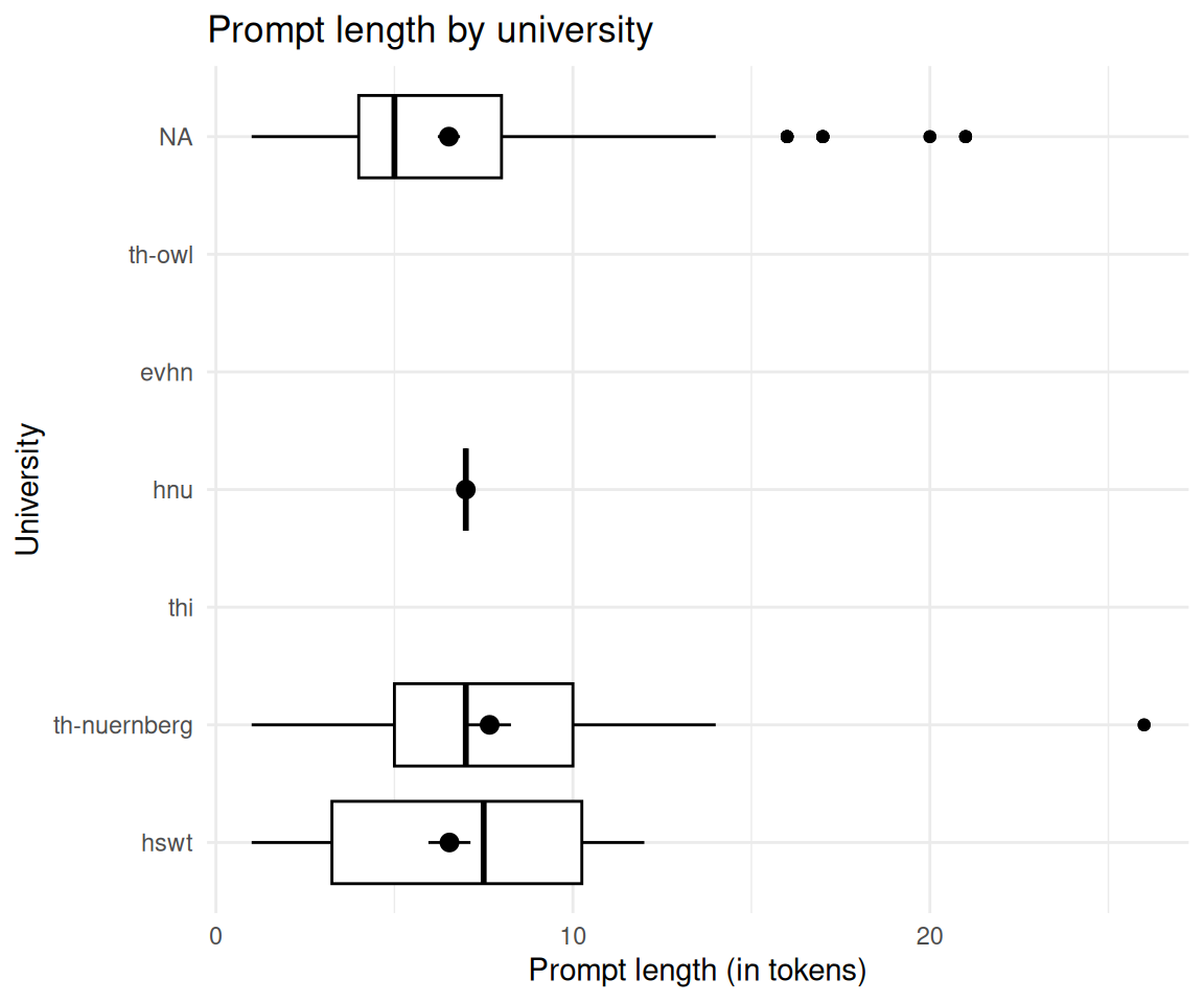

2.9 Unterscheidet sich die Token-Länge zwischen den Modulen?

prompt_length_date_uni_course |>
  group_by(course) |>
  describe_distribution(token_length) |>
  print_md()

course	Variable	Mean	SD	IQR	Range	Skewness	Kurtosis	n	n_Missing
bare	token_length	7.00	0.00	0	(7.00, 7.00)			6	8
bio	token_length				(Inf, -Inf)			0	4
cta1	token_length	6.54	4.08	9	(1.00, 12.00)	-0.15	-1.47	48	830
daba	token_length				(Inf, -Inf)			0	2
etechde	token_length				(Inf, -Inf)			0	1
fodesoa	token_length				(Inf, -Inf)			0	56
fosaq	token_length				(Inf, -Inf)			0	22
gdi	token_length				(Inf, -Inf)			0	22
gesoa	token_length	7.65	4.96	5	(1.00, 26.00)	1.63	4.41	62	659
mat11akzg	token_length				(Inf, -Inf)			0	2
nlp	token_length	8.00	3.46	6	(5.00, 11.00)	0.00	-6.00	4	65
softa	token_length				(Inf, -Inf)			0	4
thesoa	token_length				(Inf, -Inf)			0	7
wirkori	token_length				(Inf, -Inf)			0	4
zemiws	token_length				(Inf, -Inf)			0	1

2.10 Unterscheidet sich die Token-Länge im Zeitverlauf?

prompt_length_date_uni_course |>
  group_by(floor_date_month) |>
  describe_distribution(token_length) |>
  print_md()

floor_date_month	Variable	Mean	SD	IQR	Range	Skewness	Kurtosis	n	n_Missing
2025-03-01	token_length	8.03	5.88	8.00	(1.00, 21.00)	0.79	-0.36	62	488
2025-04-01	token_length	6.16	3.68	4.00	(1.00, 17.00)	0.77	0.24	191	978
2025-05-01	token_length	6.38	2.77	5.00	(3.00, 11.00)	0.26	-1.47	37	546
2025-06-01	token_length	8.72	6.69	3.00	(1.00, 26.00)	1.33	1.77	29	315
2025-07-01	token_length	6.20	2.62	2.50	(4.00, 11.00)	1.50	0.86	10	427

# Calculate limits properly
filtered_data <- prompt_length_date_uni_course |>
  filter(!is.na(floor_date_month)) |>
  mutate(floor_date_month_date = as.Date(floor_date_month))

lim <- c(
  min(filtered_data$floor_date_month_date, na.rm = TRUE),
  max(filtered_data$floor_date_month_date, na.rm = TRUE)
)

# Now create the plot
filtered_data |>
  ggplot(aes(x = floor_date_month_date, y = token_length)) +
  geom_violin(aes(group = floor_date_month_date)) +
  stat_summary(fun = "mean", geom = "point") +
  stat_summary(fun.data = "mean_se", geom = "errorbar", width = 0.2) +
  theme_minimal() +
  labs(
    title = "Prompt length over time",
    x = "Date",
    y = "Prompt length (in tokens)",
    caption = "The dots represent the mean and the error bars the standard error of the mean."
  ) +
  scale_x_date(limits = lim, labels = scales::label_date_short())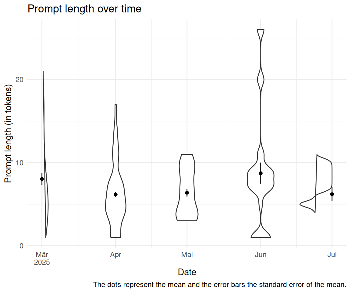

2.11 Wie oft wird wird auf ein Wort im LLM-Transkript geklickt?

data_separated_filtered |>
  filter(type == "subtitle") |>
  # rm empty rows:
  filter(!is.na(value) & value != "") |>
  count(click_transcript_word = str_detect(value, "click_transcript_word")) |>
  mutate(prop = round(n / sum(n), 2)) |>
  gt()

click_transcript_word	n	prop
FALSE	227934	1
TRUE	557	0

2.12 Wie verändert sich dieser Wert im Zeitverlauf?

click_transcript_word_per_month <-
  data_separated_filtered |>
  # rm all groups WITHOUT "click_transcript_word":
  group_by(idvisit) |>
  filter(!any(value = str_detect(value, "click_transcript_word"))) |>
  ungroup() |>
  mutate(date_visit = ymd_hms(value)) |>
  mutate(month_visit = floor_date(date_visit, unit = "month")) |>
  drop_na(date_visit) |>
  group_by(idvisit) |>
  slice(1) |>
  ungroup() |>
  count(month_visit)

click_transcript_word_per_month

rect_data_word_per_month <- comp_semester_rects(
  click_transcript_word_per_month,
  col_date = "month_visit"
)

click_transcript_word_per_month |>
  ggplot(aes(x = month_visit, y = n)) +
  geom_rect(
    data = rect_data,
    aes(xmin = xmin, xmax = xmax, ymin = ymin, ymax = Inf),
    fill = "grey",
    alpha = 0.2,
    inherit.aes = FALSE # Essential to use the rect_data columns
  ) +
  geom_line() +
  geom_smooth(method = "loess", se = FALSE, color = "blue", alpha = 0.7) +
  scale_x_date(labels = scales::label_date_short())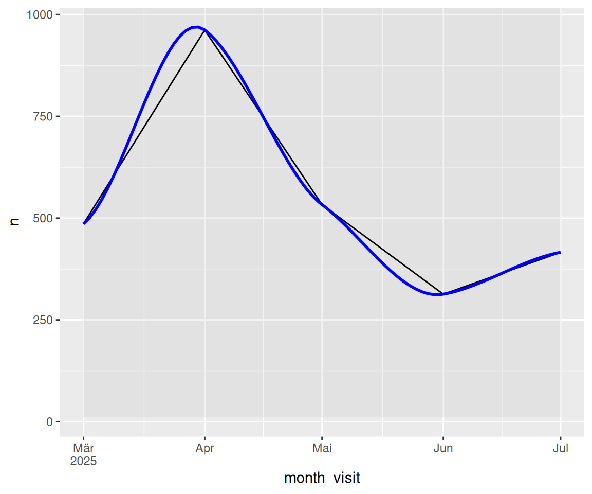

2.13 Wie lang ist der Output des LLMs (in Tokens)?

2.13.1 De vs. En

llm_response_text |>
  count(lang) |>
  mutate(prob = n / sum(n))

2.13.2 Verteilung der Anzahl der Tokens

llm_response_text |>
  describe_distribution(select = "tokens_n") |>
  print_md()

Variable	Mean	SD	IQR	Range	Skewness	Kurtosis	n	n_Missing
tokens_n	184.14	104.40	155.50	(11.00, 656.00)	0.45	0.31	397	0

2.14 Gruppieren Sie die Länge des Outputs des LLMs nach Kunden (Hochschulen).

llm_response_text_date_course_uni |>
  group_by(university) |>
  describe_distribution(select = "tokens_n")

llm_response_text_date_course_uni |>
  ggboxplot(
    x = "university",
    y = "tokens_n",
    add = "mean_se"
  ) +
  theme_minimal() +
  labs(
    title = "Number of tokens in LLM responses by university",
    x = "University",
    y = "Number of tokens"
  ) +
  coord_flip()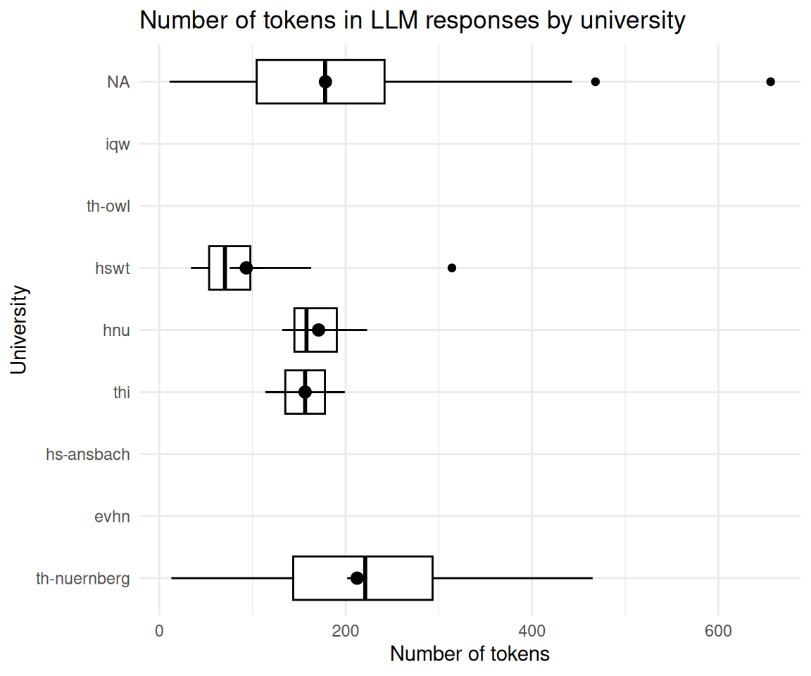

2.15 Anzahl der Token nach Kursen

llm_response_text_date_course_uni |>
  group_by(course) |>
  describe_distribution(select = "tokens_n") |>
  print_md()

course	Variable	Mean	SD	IQR	Range	Skewness	Kurtosis	n	n_Missing
anis2	tokens_n				(Inf, -Inf)			0	43
armeufa	tokens_n				(Inf, -Inf)			0	2
bare	tokens_n	171.00	46.87	91.00	(132.00, 223.00)	1.15	-1.50	3	12
bio	tokens_n				(Inf, -Inf)			0	168
biotech	tokens_n				(Inf, -Inf)			0	127
biovete	tokens_n				(Inf, -Inf)			0	244
cta1	tokens_n	93.38	71.24	72.75	(34.00, 314.00)	2.27	5.78	16	1101
daba	tokens_n	173.00		0.00	(173.00, 173.00)			1	197
enerbi	tokens_n				(Inf, -Inf)			0	10
epsy	tokens_n				(Inf, -Inf)			0	1
etechde	tokens_n				(Inf, -Inf)			0	3
fodesoa	tokens_n	256.00		0.00	(256.00, 256.00)			1	324
fomesoa	tokens_n				(Inf, -Inf)			0	6
fosaq	tokens_n				(Inf, -Inf)			0	60
gdi	tokens_n	185.00	5.00	10.00	(180.00, 190.00)	0.00	-1.50	3	47
gemwesa	tokens_n				(Inf, -Inf)			0	57
gesoa	tokens_n	186.41	126.56	217.00	(13.00, 450.00)	0.36	-1.02	64	2319
kore	tokens_n				(Inf, -Inf)			0	3
mat11akzg	tokens_n				(Inf, -Inf)			0	2
mibio	tokens_n				(Inf, -Inf)			0	206
mioek	tokens_n	156.50	60.10	85.00	(114.00, 199.00)	0.00	-2.00	2	435
nlp	tokens_n	356.50	153.44	217.00	(248.00, 465.00)	0.00	-2.00	2	65
quame1	tokens_n				(Inf, -Inf)			0	3
quanch	tokens_n				(Inf, -Inf)			0	34
softa	tokens_n				(Inf, -Inf)			0	4
thesoa	tokens_n	249.38	73.66	106.00	(15.00, 394.00)	-0.87	1.23	39	273
wirkori	tokens_n				(Inf, -Inf)			0	5
wisoa	tokens_n				(Inf, -Inf)			0	33
zemiws	tokens_n				(Inf, -Inf)			0	1

llm_response_text_date_course_uni |>
  ggboxplot(
    x = "course",
    y = "tokens_n",
    add = "mean_se"
  ) +
  theme_minimal() +
  labs(
    title = "Number of tokens in LLM responses by course",
    x = "Course",
    y = "Number of tokens"
  ) +
  coord_flip()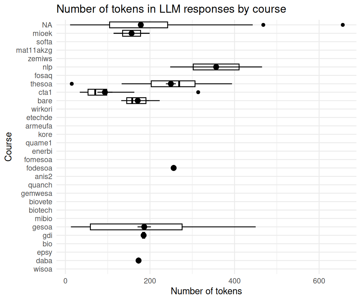

2.16 sessionInfo

sessioninfo::session_info()
## ─ Session info ───────────────────────────────────────────────────────────────
##  setting  value
##  version  R version 4.5.1 (2025-06-13)
##  os       Ubuntu 25.10
##  system   x86_64, linux-gnu
##  ui       X11
##  language (EN)
##  collate  de_DE.UTF-8
##  ctype    de_DE.UTF-8
##  tz       Europe/Berlin
##  date     2025-12-21
##  pandoc   3.6.3 @ /snap/rstudio/25/resources/app/bin/quarto/bin/tools/x86_64/ (via rmarkdown)
##  quarto   1.7.32 @ /snap/rstudio/25/resources/app/bin/quarto/bin/quarto
## 
## ─ Packages ───────────────────────────────────────────────────────────────────
##  package      * version  date (UTC) lib source
##  abind          1.4-8    2024-09-12 [3] CRAN (R 4.4.1)
##  backports      1.5.0    2024-05-23 [3] CRAN (R 4.4.1)
##  base64url      1.4      2018-05-14 [3] CRAN (R 4.0.1)
##  bayestestR   * 0.17.0   2025-08-29 [1] RSPM (R 4.5.1)
##  broom          1.0.10   2025-09-13 [1] RSPM
##  callr          3.7.6    2024-03-25 [3] CRAN (R 4.4.0)
##  car            3.1-3    2024-09-27 [3] CRAN (R 4.4.1)
##  carData        3.0-5    2022-01-06 [3] CRAN (R 4.1.2)
##  cli            3.6.5    2025-04-23 [1] CRAN (R 4.5.1)
##  coda           0.19-4.1 2024-01-31 [1] RSPM
##  codetools      0.2-20   2024-03-31 [4] CRAN (R 4.3.3)
##  correlation  * 0.8.8    2025-07-08 [1] RSPM (R 4.5.1)
##  data.table     1.17.8   2025-07-10 [1] RSPM (R 4.5.1)
##  datawizard   * 1.3.0    2025-10-11 [1] RSPM (R 4.5.1)
##  dichromat      2.0-0.1  2022-05-02 [3] CRAN (R 4.2.0)
##  digest         0.6.39   2025-11-19 [1] CRAN (R 4.5.1)
##  dplyr        * 1.1.4    2023-11-17 [3] CRAN (R 4.4.2)
##  easystats    * 0.7.5    2025-07-11 [1] RSPM (R 4.5.1)
##  effectsize   * 1.0.1    2025-05-27 [1] RSPM (R 4.5.1)
##  emmeans        1.10.7   2025-01-31 [3] CRAN (R 4.4.2)
##  estimability   1.5.1    2024-05-12 [3] CRAN (R 4.4.2)
##  evaluate       1.0.5    2025-08-27 [1] CRAN (R 4.5.1)
##  farver         2.1.2    2024-05-13 [3] CRAN (R 4.4.1)
##  fastmap        1.2.0    2024-05-15 [3] CRAN (R 4.4.1)
##  forcats      * 1.0.0    2023-01-29 [3] CRAN (R 4.2.2)
##  Formula        1.2-5    2023-02-24 [3] CRAN (R 4.2.2)
##  fs             1.6.6    2025-04-12 [1] CRAN (R 4.5.1)
##  generics       0.1.4    2025-05-09 [1] CRAN (R 4.5.1)
##  ggplot2      * 4.0.1    2025-11-14 [1] RSPM (R 4.5.1)
##  ggpubr       * 0.6.2    2025-10-17 [1] RSPM
##  ggsignif       0.6.4    2022-10-13 [3] CRAN (R 4.2.2)
##  glue           1.8.0    2024-09-30 [3] CRAN (R 4.4.2)
##  gt           * 1.1.0    2025-09-23 [1] RSPM (R 4.5.1)
##  gtable         0.3.6    2024-10-25 [3] CRAN (R 4.4.2)
##  hms            1.1.3    2023-03-21 [3] CRAN (R 4.3.1)
##  htmltools      0.5.8.1  2024-04-04 [3] CRAN (R 4.4.0)
##  htmlwidgets    1.6.4    2023-12-06 [3] CRAN (R 4.3.2)
##  igraph         2.1.4    2025-01-23 [3] CRAN (R 4.5.0)
##  insight      * 1.4.2    2025-09-02 [1] RSPM (R 4.5.1)
##  jsonlite       2.0.0    2025-03-27 [1] CRAN (R 4.5.1)
##  knitr        * 1.50     2025-03-16 [3] CRAN (R 4.4.3)
##  labeling       0.4.3    2023-08-29 [3] CRAN (R 4.3.1)
##  lattice        0.22-7   2025-04-02 [4] CRAN (R 4.4.3)
##  lifecycle      1.0.4    2023-11-07 [3] CRAN (R 4.3.2)
##  lubridate    * 1.9.4    2024-12-08 [3] CRAN (R 4.4.2)
##  magrittr       2.0.4    2025-09-12 [1] CRAN (R 4.5.1)
##  MASS           7.3-65   2025-02-28 [4] CRAN (R 4.4.3)
##  Matrix         1.7-3    2025-03-11 [4] CRAN (R 4.4.3)
##  mgcv           1.9-3    2025-04-04 [4] CRAN (R 4.4.3)
##  modelbased   * 0.13.0   2025-08-30 [1] RSPM (R 4.5.1)
##  multcomp       1.4-28   2025-01-29 [3] CRAN (R 4.4.2)
##  mvtnorm        1.3-3    2025-01-10 [1] RSPM
##  nlme           3.1-168  2025-03-31 [4] CRAN (R 4.4.3)
##  parameters   * 0.28.2   2025-09-10 [1] RSPM (R 4.5.1)
##  performance  * 0.15.2   2025-10-06 [1] RSPM (R 4.5.1)
##  pillar         1.11.1   2025-09-17 [1] CRAN (R 4.5.1)
##  pkgconfig      2.0.3    2019-09-22 [3] CRAN (R 4.0.1)
##  prettyunits    1.2.0    2023-09-24 [3] CRAN (R 4.3.1)
##  processx       3.8.6    2025-02-21 [3] CRAN (R 4.4.3)
##  ps             1.9.0    2025-02-18 [3] CRAN (R 4.4.3)
##  purrr        * 1.2.0    2025-11-04 [1] RSPM (R 4.5.1)
##  R6             2.6.1    2025-02-15 [3] CRAN (R 4.4.3)
##  RColorBrewer   1.1-3    2022-04-03 [3] CRAN (R 4.2.0)
##  readr        * 2.1.6    2025-11-14 [1] RSPM
##  report       * 0.6.2    2025-11-03 [1] RSPM (R 4.5.1)
##  rlang          1.1.6    2025-04-11 [1] CRAN (R 4.5.1)
##  rmarkdown      2.30     2025-09-28 [1] RSPM (R 4.5.1)
##  rstatix        0.7.2    2023-02-01 [3] CRAN (R 4.2.2)
##  rstudioapi     0.17.1   2024-10-22 [3] CRAN (R 4.4.1)
##  S7             0.2.1    2025-11-14 [1] RSPM (R 4.5.1)
##  sandwich       3.1-1    2024-09-15 [3] CRAN (R 4.4.1)
##  sass           0.4.10   2025-04-11 [1] RSPM (R 4.5.1)
##  scales       * 1.4.0    2025-04-24 [1] RSPM (R 4.5.1)
##  secretbase     1.0.5    2025-03-04 [1] RSPM
##  see          * 0.12.0   2025-09-14 [1] RSPM (R 4.5.1)
##  sessioninfo    1.2.3    2025-02-05 [3] CRAN (R 4.4.3)
##  stringi        1.8.7    2025-03-27 [1] CRAN (R 4.5.1)
##  stringr      * 1.6.0    2025-11-04 [1] CRAN (R 4.5.1)
##  survival       3.8-3    2024-12-17 [4] CRAN (R 4.4.2)
##  targets      * 1.11.4   2025-09-13 [1] RSPM
##  TH.data        1.1-3    2025-01-17 [3] CRAN (R 4.4.2)
##  tibble       * 3.3.0    2025-06-08 [1] CRAN (R 4.5.1)
##  tidyr        * 1.3.1    2024-01-24 [3] CRAN (R 4.3.2)
##  tidyselect     1.2.1    2024-03-11 [3] CRAN (R 4.4.0)
##  tidyverse    * 2.0.0    2023-02-22 [3] CRAN (R 4.4.2)
##  timechange     0.3.0    2024-01-18 [3] CRAN (R 4.4.3)
##  tinytable    * 0.15.1   2025-11-02 [1] CRAN (R 4.5.1)
##  tzdb           0.5.0    2025-03-15 [3] CRAN (R 4.4.3)
##  vctrs          0.6.5    2023-12-01 [3] CRAN (R 4.3.2)
##  withr          3.0.2    2024-10-28 [3] CRAN (R 4.4.1)
##  xfun           0.54     2025-10-30 [1] CRAN (R 4.5.1)
##  xml2           1.5.0    2025-11-17 [1] CRAN (R 4.5.1)
##  xtable         1.8-4    2019-04-21 [3] CRAN (R 4.0.1)
##  yaml           2.3.10   2024-07-26 [3] CRAN (R 4.4.1)
##  zoo            1.8-14   2025-04-10 [3] CRAN (R 4.4.3)
## 
##  [1] /home/sebastian-sauer/R/x86_64-pc-linux-gnu-library/4.5
##  [2] /usr/local/lib/R/site-library
##  [3] /usr/lib/R/site-library
##  [4] /usr/lib/R/library
##  * ── Packages attached to the search path.
## 
## ──────────────────────────────────────────────────────────────────────────────

Wiederverwendung

MIT

Zitat

Mit BibTeX zitieren:

@online{sauer,
  author = {Sauer, Sebastian},
  title = {Challenge 07 -\/- Solution},
  url = {https://sebastiansauer.github.io/hans-hackathon2025/challenge07-solution.html},
  langid = {de-DE}
}

Bitte zitieren Sie diese Arbeit als:

Sauer, Sebastian. n.d. “Challenge 07 -- Solution.” https://sebastiansauer.github.io/hans-hackathon2025/challenge07-solution.html.