Challenge 08 – Solution

Datum/Uhrzeit: 2026-01-09 22:46

“Eine Hackathon-Variante zur Evaluation der Klickdaten des KI-Tools ‘HaNS’”

Autor:in

Sebastian Sauer

Betrachten Sie dazu die Targets-Datei auf Github.

1 Setup

1.1 Libs

1.2 Other setup

source("_common.r")
list.files("funs", full.names = TRUE) |>
  purrr::walk(source)

options(digits = 3)
options(tinytable_tt_digits = 2)

1.3 Load Targets

tar_load(c(
  n_action_type,
  time_visit_wday,
  data_separated_distinct_slice,
  glotzdauer_prepped,
  course_and_uni_per_visit
))

2 Musterlösung

2.1 Werten Sie die Top-10-Tätigkeiten aus, die die Besucher (idvisit) auf der Website durchführen.

Tipp: Zählen Sie dafür, welche Werte wie oft bei subtitle stehen. Auf welchem Platz steht Videonutzung?

Vgl. auch https://sebastiansauer.github.io/hans/40-nutzungsarten.html?q=top#h%C3%A4ufigkeiten.

2.1.1 Insgesamt

n_action_type_counted <-
  n_action_type |>
  drop_na() |>
  count(category, sort = TRUE) |>
  mutate(prop = round(n / sum(n), 2)) |> 
  mutate(position = row_number()) |>
  select(position, everything()) 

n_action_type_counted |>
  gt()

position	category	n	prop
1	video	188539	0.88
2	visit_page	15002	0.07
3	Media item	6439	0.03
4	login	2402	0.01
5	GESOA	387	0.00
6	in_media_search	378	0.00
7	Medien	287	0.00
8	logout	212	0.00
9	Search Results Count	188	0.00
10	click_channelcard	187	0.00
11	click_topic	176	0.00
12	Kanäle	173	0.00
13	Evaluation	10	0.00
14	Data protection	4	0.00

Video steht auf Platz 1.

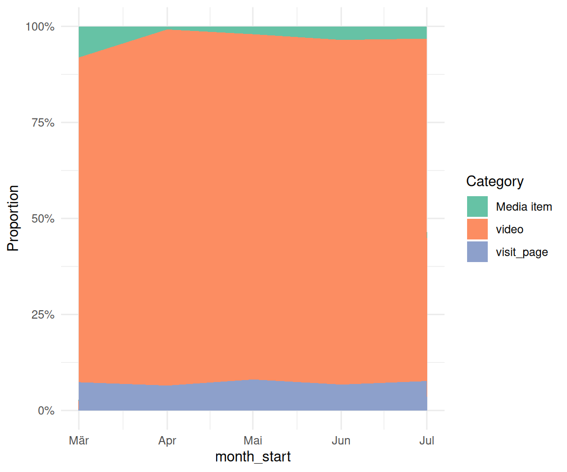
2.1.2 Bonus: Veränderung der TOP-3-Tätigkeiten im Zeitverlauf

TOP-3-Tätigkeiten:

top3 <- 
  n_action_type_counted$category[1:3] 

top3
## [1] "video"      "visit_page" "Media item"

n_action_type_per_month_top3 <-
  n_action_type |>
  select(nr, idvisit, category) |>
  ungroup() |>
  filter(category %in% top3) |>
  left_join(time_visit_wday |> ungroup()) |>
  select(-c(dow, hour, nr)) |>
  drop_na() |>
  mutate(month_start = floor_date(date_time, "month")) |>
  count(month_start, category)

n_action_type_per_month_top3 |> 
  gt()

month_start	category	n
2025-03-01	Media item	3198
2025-03-01	video	33300
2025-03-01	visit_page	2902
2025-04-01	Media item	619
2025-04-01	video	71493
2025-04-01	visit_page	5006
2025-05-01	Media item	780
2025-05-01	video	34387
2025-05-01	visit_page	3088
2025-06-01	Media item	857
2025-06-01	video	21794
2025-06-01	visit_page	1638
2025-07-01	Media item	985
2025-07-01	video	27565
2025-07-01	visit_page	2368

Vis:

n_action_type_per_month_top3 |>
  ggplot(aes(
    x = month_start,
    y = n,
    fill = category # Changed from 'color' to 'fill'
  )) +
  # Use geom_area() and set position="fill" to stack and normalize to 100%
  geom_area(position = "fill") +

  # Optional: Customize the y-axis to show percentages
  scale_y_continuous(labels = scales::label_percent()) +

  labs(
    y = "Proportion",
    fill = "Category"
  )

2.2 Berechnen Sie die Videonutzung (“Glotzdauer”)

Berechnen Sie die Videonutzung (“Glotzdauer”), d.h. die Zeit, wie lange die Besucher (idvisit) sich Videos anschauen. Tipp: Die Videodauer lässt sich mit Hilfe von eventaction und dazu play (Beginn Video schauen) bzw. pause (Ende) annähernd berechnen. Allerdings darf man auf diese Werte keine exakten Lösungen erwarten.

Achtung: Die Videozeit ist schwierig auszuwerten: Die Nutzer beenden keine Videos, in dem sie auf “Pause” drücken, sondern indem sie andere Aktionen durchführen. Dies ist aber analytisch schwer abzubilden.

Vgl. die Definition des Targets glotzdauer in der Pipeline.

Kurz gesagt wird die Zeit-Differenz zwischen zwei aufeinander folgenden “Play” und “Pause” Aktionen berechnet.

Allerdings hat dieses Vorgehen Schwierigkeiten: Nicht immer folgt auf einem “Play” ein “Pause”. Es ist schwer auszuwerten, wann die Betrachtung eines Videos endet. Daher ist diese Analyse nur vorsichtig zu interpretieren.

Die Definition der Funktion glotzdauer.R ist online dokumentiert.

2.2.1 Insgesamt

as_tibble(data_separated_distinct_slice) |>
  drop_na() |>
  filter(first_play != Inf) |>
  head(30)

idvisit	first_play	last_pause	time_diff
6	2025-03-06 14:05:22	2025-03-06 14:10:39	317 secs
8	2025-03-06 14:05:50	2025-03-06 14:07:07	77 secs
10	2025-03-06 12:55:04	2025-03-06 12:59:27	263 secs
15	2025-03-12 07:50:27	2025-03-12 07:52:27	120 secs
16	2025-03-13 11:23:34	2025-03-13 11:28:20	286 secs
18	2025-03-14 14:25:51	2025-03-14 14:41:52	961 secs
19	2025-03-14 13:43:55	2025-03-14 13:51:06	431 secs
21	2025-03-17 21:35:40	2025-03-17 21:46:24	644 secs
23	2025-03-17 21:35:40	2025-03-17 21:46:24	644 secs
26	2025-03-18 20:45:16	2025-03-18 20:54:26	550 secs
27	2025-03-18 19:34:04	2025-03-18 19:59:19	1515 secs
32	2025-03-18 11:39:13	2025-03-18 11:40:42	89 secs
35	2025-03-19 21:46:44	2025-03-19 22:00:06	802 secs
36	2025-03-19 21:14:38	2025-03-19 21:19:01	263 secs
41	2025-03-19 15:37:15	2025-03-19 16:05:20	1685 secs
47	2025-03-20 22:24:33	2025-03-20 23:58:32	5639 secs
49	2025-03-20 23:03:38	2025-03-20 23:25:33	1315 secs
50	2025-03-20 21:27:20	2025-03-20 21:55:31	1691 secs
51	2025-03-20 20:22:23	2025-03-20 21:46:19	5036 secs
53	2025-03-20 17:59:06	2025-03-20 18:55:32	3386 secs
54	2025-03-20 18:21:45	2025-03-20 18:27:09	324 secs
56	2025-03-20 17:45:16	2025-03-20 17:46:24	68 secs
58	2025-03-20 15:50:08	2025-03-20 16:25:45	2137 secs
60	2025-03-20 13:13:26	2025-03-20 14:24:50	4284 secs
61	2025-03-20 12:02:49	2025-03-20 12:05:28	159 secs
64	2025-03-20 10:01:14	2025-03-20 10:01:53	39 secs
65	2025-03-20 09:57:28	2025-03-20 10:00:09	161 secs
69	2025-03-20 08:10:46	2025-03-20 08:13:03	137 secs
73	2025-03-20 04:36:48	2025-03-20 04:56:42	1194 secs
76	2025-03-21 22:06:46	2025-03-21 22:10:28	222 secs

data_separated_distinct_slice_summary <-
  data_separated_distinct_slice |>
  mutate(time_diff = abs(time_diff)) |>
  # without glotzdauer smaller than 10 minutes:
  filter(time_diff < 60 * 10) |>
  summarise(
    time_diff_median = median(time_diff, na.rm = TRUE),
    time_diff_median_hms = hms::as_hms(median(time_diff, na.rm = TRUE)),
    time_diff_mean_hms = hms::as_hms(mean(time_diff, na.rm = TRUE)),
    time_diff_mean = mean(time_diff, na.rm = TRUE),
    time_diff_sd = sd(time_diff, na.rm = TRUE),
    n = n()
  )

data_separated_distinct_slice_summary |> 
  kable(digits = 2)

time_diff_median	time_diff_median_hms	time_diff_mean_hms	time_diff_mean	time_diff_sd	n
148 secs	00:02:28.5	00:03:27.688889	208 secs	171	630

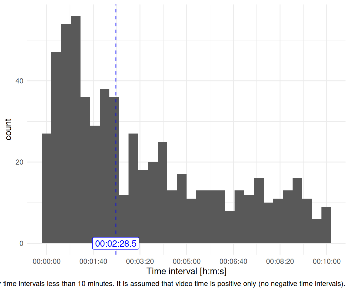
Für die folgende Darstellung wurden die absoluten Zeitwerte verwendet, d.h. ohne Vorzeichen.

data_separated_distinct_slice |>
  # we will assume that negative glotzdauer is the as positive glotzdauer:
  mutate(time_diff = abs(time_diff)) |>
  # without glotzdauer smaller than 10 minutes:
  filter(time_diff < 60 * 10) |>
  ggplot(aes(x = time_diff)) +
  geom_histogram() +
  scale_x_time(breaks = pretty_breaks()) +
  labs(
    x = "Time interval [h:m:s]",
    caption = "Only time intervals less than 10 minutes. It is assumed that video time is positive only (no negative time intervals)."
  ) +
  theme_minimal() +
  geom_vline(xintercept = data_separated_distinct_slice_summary$time_diff_median, 
  linetype = "dashed", color = "blue") +
  annotate("label",
    x = trunc(data_separated_distinct_slice_summary$time_diff_median_hms),
    y = 0,
    color = "blue",
    label = data_separated_distinct_slice_summary$time_diff_median_hms, 
  )

glotzdauer_tbl <-
  glotzdauer_prepped |>
  select(time_diff_abs_sec, time_diff_abs_min) |>
  describe_distribution()

glotzdauer_tbl |>
  print_md()

Variable	Mean	SD	IQR	Range	Skewness	Kurtosis	n	n_Missing
time_diff_abs_sec	207.69	171.25	268.25	(0.00, 599.00)	0.72	-0.70	630	0
time_diff_abs_min	3.46	2.85	4.47	(0.00, 9.98)	0.72	-0.70	630	0

glotzdauer_tbl |>
  mutate(across(where(is.numeric), ~ round(., 2))) |>
  ggpubr::ggtexttable()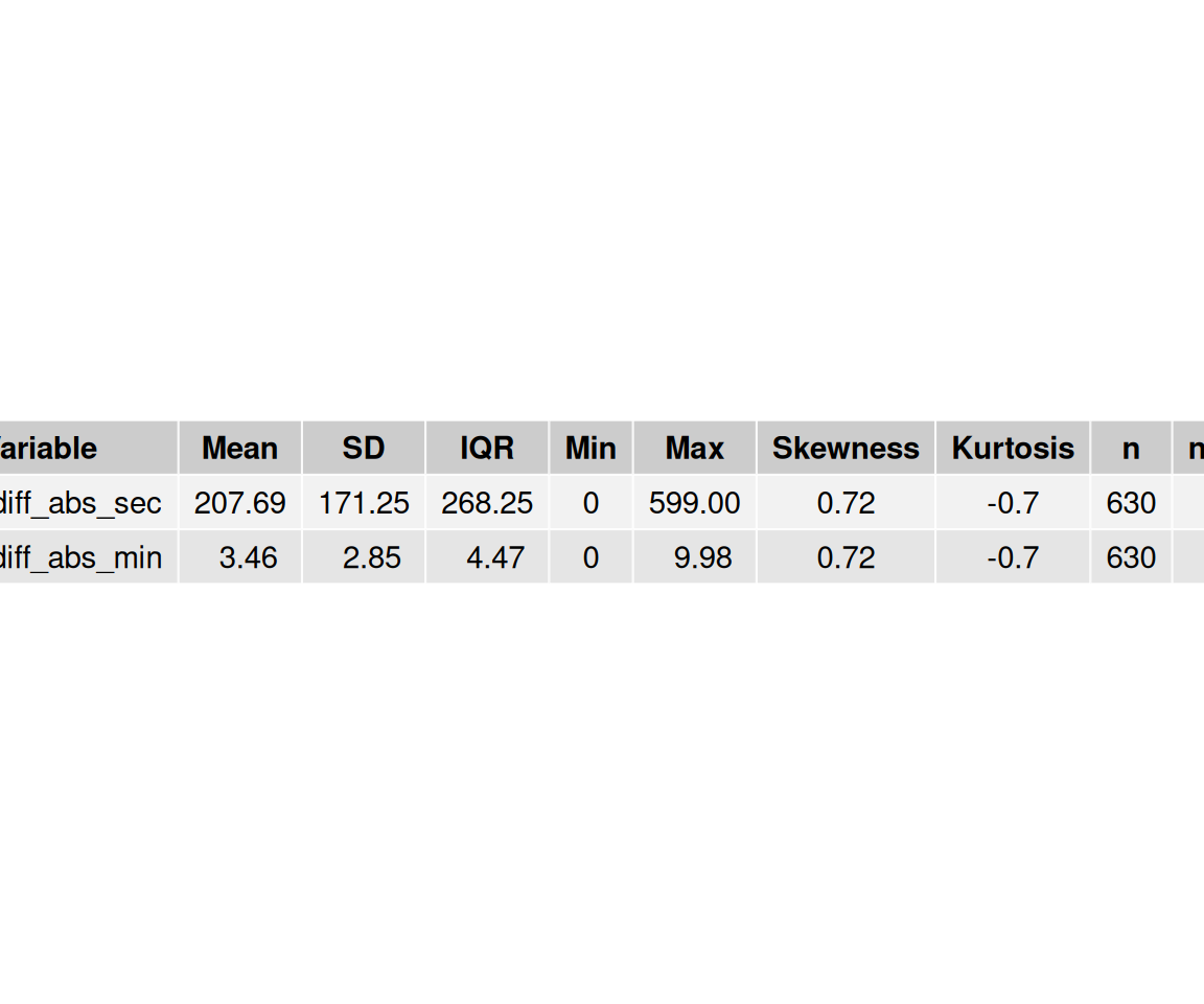

2.3 Untersuchen und visualisieren Sie, ob sich das Verhalten in Bezug auf die Videos verändert hat im Laufe der Zeit (Wochen und Monate) im Hinblick auf die Glotzdauer.

2.3.1 Wochen

glotzdauer_prepped_tbl_weeks <-
  glotzdauer_prepped |>
  mutate(first_of_month = floor_date(first_play, unit = "week")) |>
  group_by(first_of_month) |>
  summarise(time_diff_mean = mean(time_diff, na.rm = TRUE))

glotzdauer_prepped_tbl_weeks

first_of_month	time_diff_mean
2025-03-03	219 secs
2025-03-10	279 secs
2025-03-17	241 secs
2025-03-24	175 secs
2025-03-31	212 secs
2025-04-07	229 secs
2025-04-14	225 secs
2025-04-21	227 secs
2025-04-28	175 secs
2025-05-05	201 secs
2025-05-12	192 secs
2025-05-19	207 secs
2025-05-26	182 secs
2025-06-02	234 secs
2025-06-09	282 secs
2025-06-16	154 secs
2025-06-23	158 secs
2025-06-30	216 secs
2025-07-07	200 secs
2025-07-14	275 secs

glotzdauer_prepped_tbl_weeks |>
  ggplot(aes(x = first_of_month, y = time_diff_mean)) +
  geom_line() +
  theme_minimal() +
  geom_smooth(method = "loess", se = FALSE, color = "blue") +
  labs(
    x = "Date",
    y = "Average video watching time [s]"
  )

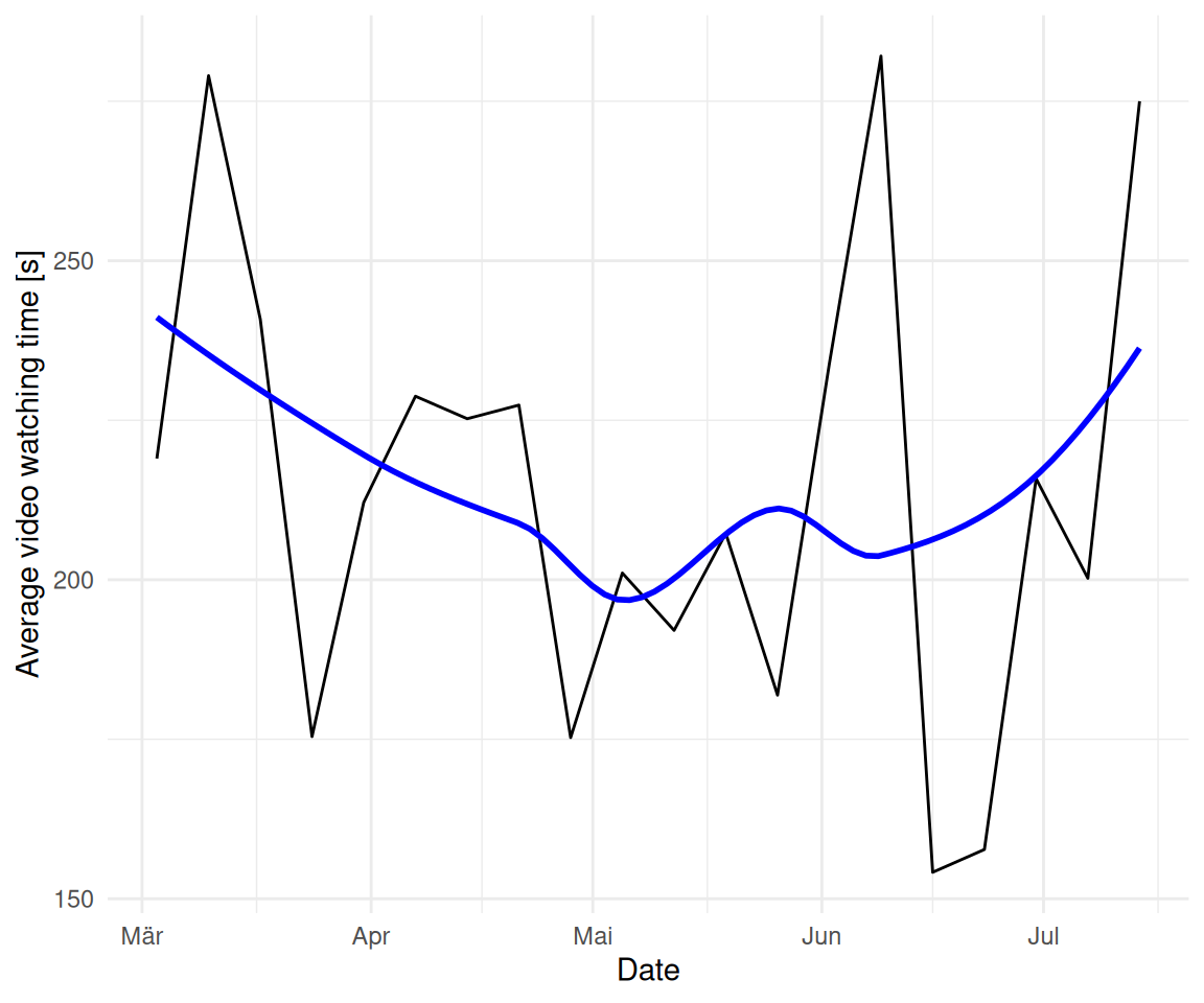
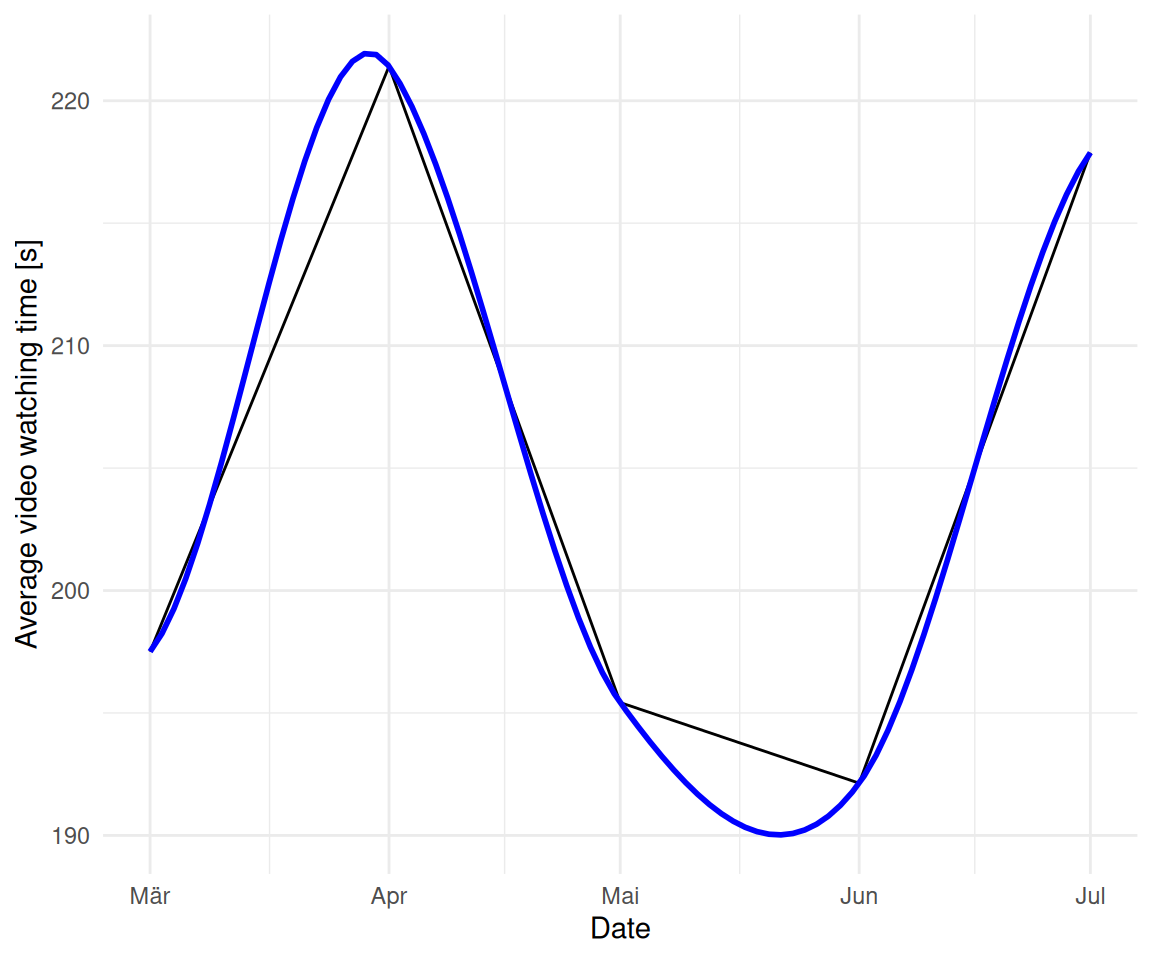
2.3.2 Monate

glotzdauer_prepped_tbl <-
  glotzdauer_prepped |>
  mutate(first_of_month = floor_date(first_play, unit = "month")) |>
  group_by(first_of_month) |>
  summarise(time_diff_mean = mean(time_diff, na.rm = TRUE))

glotzdauer_prepped_tbl

first_of_month	time_diff_mean
2025-03-01	198 secs
2025-04-01	221 secs
2025-05-01	195 secs
2025-06-01	192 secs
2025-07-01	218 secs

glotzdauer_prepped_tbl |>
  ggplot(aes(x = first_of_month, y = time_diff_mean)) +
  geom_line() +
  theme_minimal() +
  geom_smooth(method = "loess", se = FALSE, color = "blue") +
  labs(
    x = "Date",
    y = "Average video watching time [s]"
  )

2.4 Berechnen Sie die Videonutzung pro Kunde (Hochschule).


glotzdauer_per_customer <-
  glotzdauer_prepped |>
  left_join(
    course_and_uni_per_visit |>
      select(idvisit, university) |>
      distinct() |> 
      mutate(idvisit = as.integer(idvisit)),
  ) |>
  group_by(university) |>
  summarise(
    time_diff_mean = mean(time_diff, na.rm = TRUE),
    time_diff_median = median(time_diff, na.rm = TRUE),
    n = n()
  ) |>
  drop_na() |> 
  arrange(desc(time_diff_mean))

glotzdauer_per_customer %>%
  mutate(
    time_diff_mean = as.difftime(round(as.numeric(time_diff_mean), 0), units = "secs"),
    time_diff_median = as.difftime(round(as.numeric(time_diff_median), 0), units = "secs")
  ) |> 
  gt()

university	time_diff_mean	time_diff_median	n
evhn	465	465	1
th-nuernberg	217	158	150
hswt	209	169	236
th-owl	74	74	1

2.5 Zum Quarto-Bericht

2.5.1 Wie kann man die Größe eines Diagramms in Quarto einstellen?

2.5.2 Wie kann man Diagramme referenzieren (z.B. “Diagramm <3> zeigt blabla”, wobei “Diagramm 3” verlinkt ist zum Diagramm).

https://quarto.org/docs/authoring/cross-references.html

2.5.3 Wie kann man eine Gliederung zum Quarto-Bericht hinzufügen.

https://quarto.org/docs/reference/formats/html.html

2.5.4 Welche Code-Chunk-Optionen gibt es in Quarto? Nennen Sie zumindest 3. Wie ist die Syntax aufgebaut?

https://quarto.org/docs/reference/cells/cells-knitr.html

2.5.5 Beschreiben Sie das Ausgabeformat “Typst”

2.6 sessionInfo

sessioninfo::session_info()
## ─ Session info ───────────────────────────────────────────────────────────────
##  setting  value
##  version  R version 4.5.1 (2025-06-13)
##  os       Ubuntu 25.10
##  system   x86_64, linux-gnu
##  ui       X11
##  language (EN)
##  collate  de_DE.UTF-8
##  ctype    de_DE.UTF-8
##  tz       Europe/Berlin
##  date     2026-01-09
##  pandoc   3.6.3 @ /usr/lib/rstudio/resources/app/bin/quarto/bin/tools/x86_64/ (via rmarkdown)
##  quarto   1.8.25 @ /usr/lib/rstudio/resources/app/bin/quarto/bin/quarto
## 
## ─ Packages ───────────────────────────────────────────────────────────────────
##  package      * version  date (UTC) lib source
##  abind          1.4-8    2024-09-12 [3] CRAN (R 4.4.1)
##  backports      1.5.0    2024-05-23 [3] CRAN (R 4.4.1)
##  base64url      1.4      2018-05-14 [3] CRAN (R 4.0.1)
##  bayestestR   * 0.17.0   2025-08-29 [1] RSPM (R 4.5.1)
##  broom          1.0.10   2025-09-13 [1] RSPM
##  callr          3.7.6    2024-03-25 [3] CRAN (R 4.4.0)
##  car            3.1-3    2024-09-27 [3] CRAN (R 4.4.1)
##  carData        3.0-5    2022-01-06 [3] CRAN (R 4.1.2)
##  cli            3.6.5    2025-04-23 [1] CRAN (R 4.5.1)
##  coda           0.19-4.1 2024-01-31 [1] RSPM
##  codetools      0.2-20   2024-03-31 [4] CRAN (R 4.3.3)
##  correlation  * 0.8.8    2025-07-08 [1] RSPM (R 4.5.1)
##  cowplot        1.1.3    2024-01-22 [3] CRAN (R 4.3.2)
##  data.table     1.17.8   2025-07-10 [1] RSPM (R 4.5.1)
##  datawizard   * 1.3.0    2025-10-11 [1] RSPM (R 4.5.1)
##  dichromat      2.0-0.1  2022-05-02 [3] CRAN (R 4.2.0)
##  digest         0.6.39   2025-11-19 [1] CRAN (R 4.5.1)
##  dplyr        * 1.1.4    2023-11-17 [3] CRAN (R 4.4.2)
##  easystats    * 0.7.5    2025-07-11 [1] RSPM (R 4.5.1)
##  effectsize   * 1.0.1    2025-05-27 [1] RSPM (R 4.5.1)
##  emmeans        1.10.7   2025-01-31 [3] CRAN (R 4.4.2)
##  estimability   1.5.1    2024-05-12 [3] CRAN (R 4.4.2)
##  evaluate       1.0.5    2025-08-27 [1] CRAN (R 4.5.1)
##  farver         2.1.2    2024-05-13 [3] CRAN (R 4.4.1)
##  fastmap        1.2.0    2024-05-15 [3] CRAN (R 4.4.1)
##  forcats      * 1.0.0    2023-01-29 [3] CRAN (R 4.2.2)
##  Formula        1.2-5    2023-02-24 [3] CRAN (R 4.2.2)
##  fs             1.6.6    2025-04-12 [1] CRAN (R 4.5.1)
##  generics       0.1.4    2025-05-09 [1] CRAN (R 4.5.1)
##  ggplot2      * 4.0.1    2025-11-14 [1] RSPM (R 4.5.1)
##  ggpubr       * 0.6.2    2025-10-17 [1] RSPM
##  ggsignif       0.6.4    2022-10-13 [3] CRAN (R 4.2.2)
##  glue           1.8.0    2024-09-30 [3] CRAN (R 4.4.2)
##  gridExtra      2.3      2017-09-09 [3] CRAN (R 4.0.1)
##  gt           * 1.1.0    2025-09-23 [1] RSPM (R 4.5.1)
##  gtable         0.3.6    2024-10-25 [3] CRAN (R 4.4.2)
##  hms            1.1.3    2023-03-21 [3] CRAN (R 4.3.1)
##  htmltools      0.5.8.1  2024-04-04 [3] CRAN (R 4.4.0)
##  htmlwidgets    1.6.4    2023-12-06 [3] CRAN (R 4.3.2)
##  igraph         2.1.4    2025-01-23 [3] CRAN (R 4.5.0)
##  insight      * 1.4.2    2025-09-02 [1] RSPM (R 4.5.1)
##  jsonlite       2.0.0    2025-03-27 [1] CRAN (R 4.5.1)
##  knitr        * 1.50     2025-03-16 [3] CRAN (R 4.4.3)
##  labeling       0.4.3    2023-08-29 [3] CRAN (R 4.3.1)
##  lattice        0.22-7   2025-04-02 [4] CRAN (R 4.4.3)
##  lifecycle      1.0.4    2023-11-07 [3] CRAN (R 4.3.2)
##  lubridate    * 1.9.4    2024-12-08 [3] CRAN (R 4.4.2)
##  magrittr       2.0.4    2025-09-12 [1] CRAN (R 4.5.1)
##  MASS           7.3-65   2025-02-28 [4] CRAN (R 4.4.3)
##  Matrix         1.7-3    2025-03-11 [4] CRAN (R 4.4.3)
##  mgcv           1.9-3    2025-04-04 [4] CRAN (R 4.4.3)
##  modelbased   * 0.13.0   2025-08-30 [1] RSPM (R 4.5.1)
##  multcomp       1.4-28   2025-01-29 [3] CRAN (R 4.4.2)
##  mvtnorm        1.3-3    2025-01-10 [1] RSPM
##  nlme           3.1-168  2025-03-31 [4] CRAN (R 4.4.3)
##  parameters   * 0.28.2   2025-09-10 [1] RSPM (R 4.5.1)
##  performance  * 0.15.2   2025-10-06 [1] RSPM (R 4.5.1)
##  pillar         1.11.1   2025-09-17 [1] CRAN (R 4.5.1)
##  pkgconfig      2.0.3    2019-09-22 [3] CRAN (R 4.0.1)
##  prettyunits    1.2.0    2023-09-24 [3] CRAN (R 4.3.1)
##  processx       3.8.6    2025-02-21 [3] CRAN (R 4.4.3)
##  ps             1.9.0    2025-02-18 [3] CRAN (R 4.4.3)
##  purrr        * 1.2.0    2025-11-04 [1] RSPM (R 4.5.1)
##  R6             2.6.1    2025-02-15 [3] CRAN (R 4.4.3)
##  RColorBrewer   1.1-3    2022-04-03 [3] CRAN (R 4.2.0)
##  readr        * 2.1.6    2025-11-14 [1] RSPM
##  report       * 0.6.2    2025-11-03 [1] RSPM (R 4.5.1)
##  rlang          1.1.6    2025-04-11 [1] CRAN (R 4.5.1)
##  rmarkdown      2.30     2025-09-28 [1] RSPM (R 4.5.1)
##  rstatix        0.7.2    2023-02-01 [3] CRAN (R 4.2.2)
##  rstudioapi     0.17.1   2024-10-22 [3] CRAN (R 4.4.1)
##  S7             0.2.1    2025-11-14 [1] RSPM (R 4.5.1)
##  sandwich       3.1-1    2024-09-15 [3] CRAN (R 4.4.1)
##  sass           0.4.10   2025-04-11 [1] RSPM (R 4.5.1)
##  scales       * 1.4.0    2025-04-24 [1] RSPM (R 4.5.1)
##  secretbase     1.0.5    2025-03-04 [1] RSPM
##  see          * 0.12.0   2025-09-14 [1] RSPM (R 4.5.1)
##  sessioninfo    1.2.3    2025-02-05 [3] CRAN (R 4.4.3)
##  stringi        1.8.7    2025-03-27 [1] CRAN (R 4.5.1)
##  stringr      * 1.6.0    2025-11-04 [1] CRAN (R 4.5.1)
##  survival       3.8-3    2024-12-17 [4] CRAN (R 4.4.2)
##  targets      * 1.11.4   2025-09-13 [1] RSPM
##  TH.data        1.1-3    2025-01-17 [3] CRAN (R 4.4.2)
##  tibble       * 3.3.0    2025-06-08 [1] CRAN (R 4.5.1)
##  tidyr        * 1.3.1    2024-01-24 [3] CRAN (R 4.3.2)
##  tidyselect     1.2.1    2024-03-11 [3] CRAN (R 4.4.0)
##  tidyverse    * 2.0.0    2023-02-22 [3] CRAN (R 4.4.2)
##  timechange     0.3.0    2024-01-18 [3] CRAN (R 4.4.3)
##  tinytable    * 0.15.1   2025-11-02 [1] CRAN (R 4.5.1)
##  tzdb           0.5.0    2025-03-15 [3] CRAN (R 4.4.3)
##  vctrs          0.6.5    2023-12-01 [3] CRAN (R 4.3.2)
##  withr          3.0.2    2024-10-28 [3] CRAN (R 4.4.1)
##  xfun           0.54     2025-10-30 [1] CRAN (R 4.5.1)
##  xml2           1.5.0    2025-11-17 [1] CRAN (R 4.5.1)
##  xtable         1.8-4    2019-04-21 [3] CRAN (R 4.0.1)
##  yaml           2.3.10   2024-07-26 [3] CRAN (R 4.4.1)
##  zoo            1.8-14   2025-04-10 [3] CRAN (R 4.4.3)
## 
##  [1] /home/sebastian-sauer/R/x86_64-pc-linux-gnu-library/4.5
##  [2] /usr/local/lib/R/site-library
##  [3] /usr/lib/R/site-library
##  [4] /usr/lib/R/library
##  * ── Packages attached to the search path.
## 
## ──────────────────────────────────────────────────────────────────────────────

Wiederverwendung

MIT

Zitat

Mit BibTeX zitieren:

@online{sauer,
  author = {Sauer, Sebastian},
  title = {Challenge 08 -\/- Solution},
  url = {https://sebastiansauer.github.io/hans-hackathon2025/challenge08-solution.html},
  langid = {de-DE}
}

Bitte zitieren Sie diese Arbeit als:

Sauer, Sebastian. n.d. “Challenge 08 -- Solution.” https://sebastiansauer.github.io/hans-hackathon2025/challenge08-solution.html.