Edit: This post was updated, including two errors fixed - thanks to (private) comments from Norman Markgraf.

z-values, aka values coming from an z-transformation are a frequent creature in statistics land. Among their properties are the following:

1. mean is zero
2. variance is one (and hence sd is one)

But why is that? How come that this two properties are true? The goal of this post is to shed light on these two properties of z-values.

Mean value of z-value is zero

There are a number of ways to explain this fact.

One is that it is one feature of mean values that the sum of the differences of the mean is zero. z-values tell nothing but the difference to the mean (in relation to the SD of the distribution). Hence, once you realize that the mean z-value is nothing but some mean value, you will see that the mean of a distribution/sample in z-values equals zero.

Intuition

Look at the following codea and diagram as an intuition:

library(tidyverse)

mtcars %>% 
  select(cyl) %>% 
  slice(1:10) %>% 
  mutate(cyl_mean = mean(cyl),
         diff = cyl - cyl_mean) %>% 
  summarise(sum(diff))

##      sum(diff)
## 1 1.776357e-15

So our sum of the diff values is (practically) zero.

mtcars %>% 
  rownames_to_column %>% 
  select(cyl, rowname) %>% 
  slice(1:10) %>% 
  mutate(cyl_mean = mean(cyl),
         diff = cyl - cyl_mean,
         sign_diff = sign(diff)) %>% 
  ggplot() +
  aes(x = rowname, y = diff) +
  geom_col(aes(fill = factor(sign_diff))) +
  coord_flip() +
  guides(fill = FALSE)

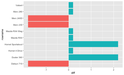
The diagram above is meant to give an impression that the negative and positive differences to the mean “cancel out”, ie., sum up to zero. Put pluntly: First, concatenate the red bars. Then, concatenate the magenta bars. You will find the total red bar and the total magenta bar are of the same length.

One further visualization:

cyl_mean <- mean(mtcars[1:10, "cyl"])

mtcars %>% 
  rownames_to_column %>% 
  select(cyl, rowname) %>% 
  slice(1:10) %>% 
  mutate(cyl_mean = mean(cyl),
         diff = cyl - cyl_mean,
         sign_diff = sign(diff),
         ID = 1:10) %>% 
  ggplot() +
  aes(x = ID, y = cyl) +
  geom_col(aes(fill = factor(sign_diff))) +
  coord_flip() +
  guides(fill = FALSE) +
  geom_hline(yintercept = cyl_mean) +
  geom_rect(aes(xmin = ID-.45, xmax = ID+.45,
                ymin = cyl_mean,
                ymax = cyl_mean + diff
               ),
            alpha = .7) +
  scale_x_continuous(breaks = 1:10)

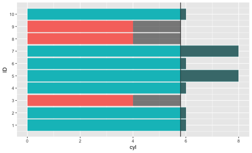
Saying that the differences of the values to the mean sum up amounts to saying that the “negative bars” (starting at the vertical mean line at about 5.8) are of equal length if concatenated as the “positive bars” (again starting at the vertical line), concatenated.

More formally

More formally, let \(X\) be some numeric variable, and \(\bar{x}\) the respective arithmetic mean, then \(\sum{(X_i - \bar{x}}) = 0\).

But why does this equation hold? And how does this apply to z-values?

Let’s look at some algebra:

\(\bar{z}_x =\) \(\frac{1}{n}\sum{z_{xi}} =\) \(\frac{1}{n}\sum{\frac{x_i- \bar{x}}{sd_x}} =\) \(\frac{1}{n} sd^-1 \underbrace{\sum{(x_i - \bar{x})}}_{\text{0}} = 0\)

But the sum of the differences to the mean (\(\sum{(x_i - \bar{x})}\)) is zero. Hence, the whole term is zero. That’s why (that’s one reason hot to explain why) the mean of z-values is zero.

But… why is the sum of differences from the mean equal to zero?

\(\sum{(x_i - \bar{x})} = \sum{x_i} - \sum{\bar{x}}=\) \(\sum{x_i} - n\bar{x} = \sum{x_i} - n \frac{\sum{x_i}}{n} = \sum{x_i} - \sum{x_i} = 0\)

SD of z-values is one

Ok, maybe the mean value of z-values is zero. But why is the SD or the variance equal to one?

If the variance is one, we will agree that the sd is one, too, because the root of 1 is 1.

Intuition

Well, suppose you take all the differences \(d\) from the mean and divide them by \(sd\). Let’s call the new differences \(d^{\prime}\). Not very surprisingly, the \(sd\) of \(d^{\prime}\) will also change accordingly - multiplied by \(sd^{-1}\), ie., \(sd^{\prime}\) will be divided by the factor \(sd\). And that yields 1.

More formally

Let \(V(X)\) be the variance (V) of some variable X, the remaining details are as above.

But, \(\bar{z}_x = 0\), as discussed above. Thus, the equation is shortened to:

Now we replace \(z_{x_i}\) by its definition.

Rearranging gives:

which can be simplified to

Thus, we see that the variance of z-values equals 1.

Similarly, picking up the idea from the intuition above, note that

In other words, if we multiply our values (the \(x_i\)s) by some factor \(a\), the resulting variance will increase by \(a^2\). In case that the mean value is zero (as for z-values), then we may say that “if we multiply our differences \(d\) by some factor \(a\), the variance will increase by \(a^2\)”. Taking the root of the variance, we are left with the sd changed by factor \(a\).