Kapitel 8 Fallstudie Normierung

library(tidyverse)
library(DataExplorer)
library(easystats)

8.1 Explorative Datenanalyse

data_url <- "https://raw.githubusercontent.com/sebastiansauer/modar/master/datasets/extra.csv"
extra <- read_csv(data_url)

extra %>% 
  select(ends_with("_mean")) %>% 
  plot_histogram()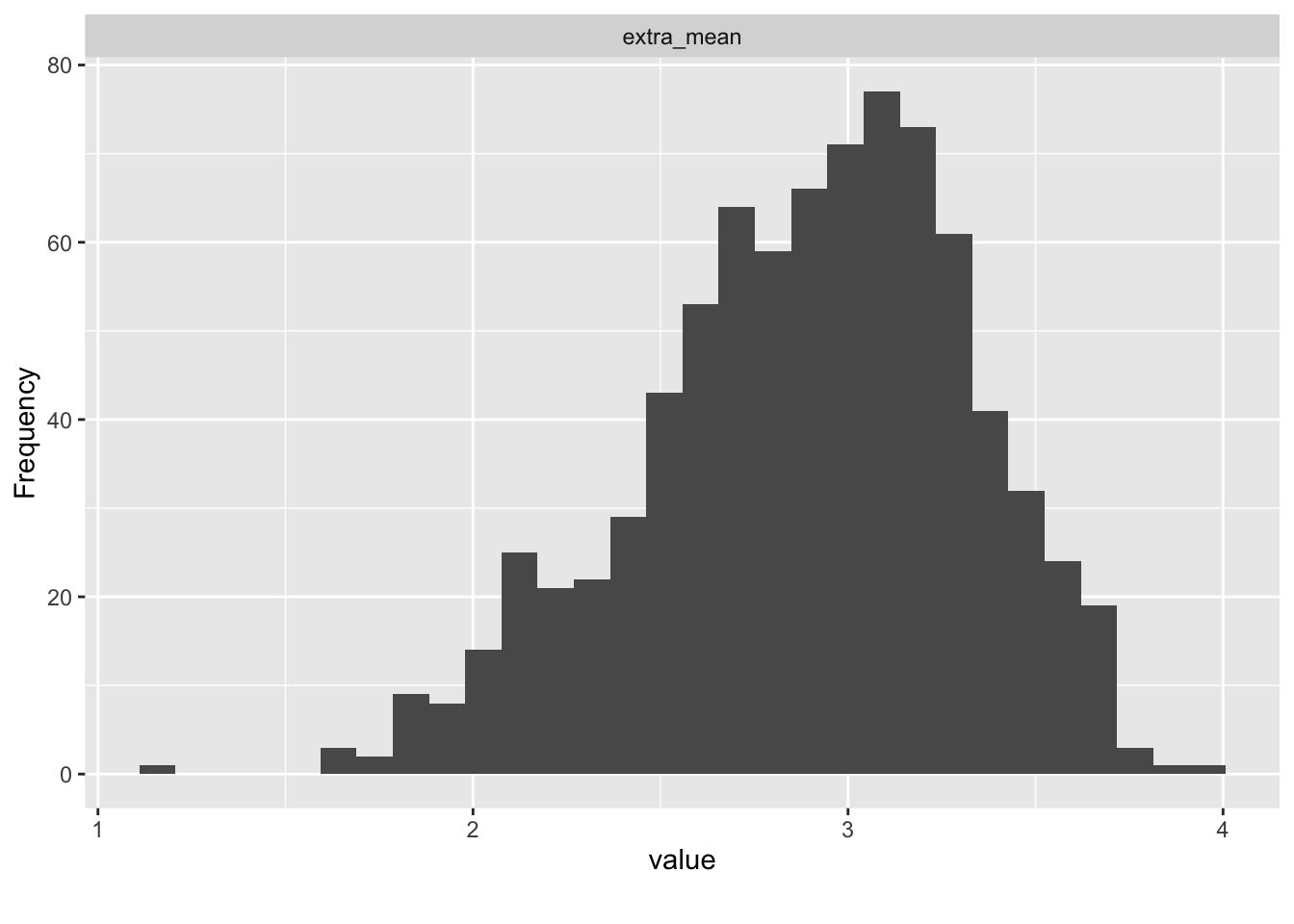

extra %>% 
  select(extra_mean, n_facebook_friends, n_hangover, age, sex, time_conversation, sleep_week, sleep_wend) %>% 
  describe_distribution()
#> Variable           |     Mean |       SD |    IQR |            Range | Skewness | Kurtosis |   n | n_Missing
#> ------------------------------------------------------------------------------------------------------------
#> extra_mean         |     2.89 |     0.45 |   0.60 |     [1.20, 4.00] |    -0.43 |    -0.11 | 822 |         4
#> n_facebook_friends |   532.61 |  3704.48 | 300.00 | [0.00, 96055.00] |    25.67 |   662.76 | 671 |       155
#> n_hangover         |     9.47 |    30.72 |   9.00 |   [0.00, 738.00] |    17.54 |   399.53 | 800 |        26
#> age                |    25.50 |     5.75 |   6.00 |   [18.00, 54.00] |     1.81 |     4.39 | 813 |        13
#> time_conversation  | 1.34e+06 | 3.65e+07 |  10.00 | [0.00, 1.00e+09] |    27.37 |   749.00 | 749 |        77
#> sleep_week         |    18.00 |    26.98 |   2.00 |    [5.00, 85.00] |     2.16 |     3.46 |  12 |       814
#> sleep_wend         |     8.25 |     1.22 |   2.75 |    [7.00, 10.00] |     0.52 |    -1.27 |  12 |       814

8.2 Normwerte berechnen

8.2.1 Hilfsfunktionen

Zwei Hilfskräfte (in Form von R-Funktionen) brauchen wir: Die erste Funktion berechnet Normwerte, s.Infos here:

convert_to_norm_value <- 
  function(score, data_vec, mu = 0, sigma = 1) {
  numerator <- (score - mean(data_vec, na.rm = TRUE))
  out <-  (numerator / sd(data_vec)) * sigma + mu
  return(out)
}

Probieren wir es aus. Aber zuerst müssen wir die NA entfernen, da das convert_to_norm_value nicht kann.

extra_drop_na <- 
extra %>% 
  select(extra_mean) %>% 
  drop_na()
  
convert_to_norm_value(score = 3, data_vec = extra_drop_na$extra_mean)
#> [1] 0.2415975

Diese Funktion wenden wir für mehrere Normierungsarten an, im Rahmen einer zweiten Funktion:

compute_all_norms <- function(x, min_score = 0, max_score = max(x), by = .5){
  
  x_ecdf <- ecdf(x)  # empircal cumulative distribution function - gives back function
  
  out <-
    tibble(
      score = seq(from = min_score, to = max_score, by = by),
      perc_rank = x_ecdf(score),
      z = map_dbl(score, ~ convert_to_norm_value(.x, data_vec = x)),
      stanine = map_dbl(score, ~ convert_to_norm_value(.x, data_vec = x, mu = 5, sigma = 2)),
      T = map_dbl(score, ~ convert_to_norm_value(.x, data_vec = x, mu = 50, sigma = 10)),
      perc_normal = map_dbl(z, pnorm)
    ) %>% 
    mutate(stanine = case_when(
      stanine > 9 ~ 9,
      stanine < 1 ~ 1,
      TRUE ~ stanine
    ))
  return(out)
}

8.2.2 Normwerte berechnen

extra %>% 
  select(ends_with("_mean")) %>% 
  drop_na() %>% 
  map(~ kable(compute_all_norms(., min_score = 1, max_score = 4, by = .1), 
                     digits = 2)) %>% 
  print()

$extra_mean

score	perc_rank	z	stanine	T	perc_normal
1.0	0.00	-4.19	1.00	8.13	0.00
1.1	0.00	-3.97	1.00	10.35	0.00
1.2	0.00	-3.74	1.00	12.56	0.00
1.3	0.00	-3.52	1.00	14.78	0.00
1.4	0.00	-3.30	1.00	16.99	0.00
1.5	0.00	-3.08	1.00	19.20	0.00
1.6	0.00	-2.86	1.00	21.42	0.00
1.7	0.01	-2.64	1.00	23.63	0.00
1.8	0.02	-2.42	1.00	25.85	0.01
1.9	0.03	-2.19	1.00	28.06	0.01
2.0	0.05	-1.97	1.06	30.28	0.02
2.1	0.08	-1.75	1.50	32.49	0.04
2.2	0.10	-1.53	1.94	34.70	0.06
2.3	0.12	-1.31	2.38	36.92	0.10
2.4	0.16	-1.09	2.83	39.13	0.14
2.5	0.21	-0.87	3.27	41.35	0.19
2.6	0.28	-0.64	3.71	43.56	0.26
2.7	0.36	-0.42	4.15	45.77	0.34
2.8	0.43	-0.20	4.60	47.99	0.42
2.9	0.51	0.02	5.04	50.20	0.51
3.0	0.60	0.24	5.48	52.42	0.60
3.1	0.69	0.46	5.93	54.63	0.68
3.2	0.78	0.68	6.37	56.84	0.75
3.3	0.85	0.91	6.81	59.06	0.82
3.4	0.90	1.13	7.25	61.27	0.87
3.5	0.94	1.35	7.70	63.49	0.91
3.6	0.97	1.57	8.14	65.70	0.94
3.7	0.99	1.79	8.58	67.91	0.96
3.8	1.00	2.01	9.00	70.13	0.98
3.9	1.00	2.23	9.00	72.34	0.99
4.0	1.00	2.46	9.00	74.56	0.99

Bühner, M. 2011. Einführung in Die Test- Und Fragebogenkonstruktion. PS Psychologie. Hallbergmoos: Pearson Studium. https://books.google.de/books?id=Y4990CfV3wgC.

Lienert, Gustav A., and Ulrich Raatz. 1998. Testaufbau Und Testanalyse. 6. Auflage. Weinheim: Beltz, Psychologie Verlags Union.

Mair, Patrick. 2018. Modern Psychometrics with r. New York, NY: Springer Science+Business Media.

Satow, L. 2012. “SCI - Stress- und Coping-Inventar.” https://doi.org/10.23668/PSYCHARCHIVES.4604.

———. 2020. “B5T®. Big-Five-Persönlichkeitstest.” https://doi.org/10.23668/PSYCHARCHIVES.4611.

Sauer, Sebastian. 2019. Moderne Datenanalyse Mit r: Daten Einlesen, Aufbereiten, Visualisieren Und Modellieren. 1. Auflage 2019. FOM-Edition. Wiesbaden: Springer. https://www.springer.com/de/book/9783658215866.

Steyer, Rolf, and Michael Eid. 1993. Messen Und Testen. Heidelberg: Springer.

7 Itemanalyse