I kept wondering who to plot two R plots side by side (ie., in one “row”) in a .Rmd chunk. Here’s a way, well actually a number of ways, some good, some … not.

library(tidyverse)
library(gridExtra)
library(grid)
library(png)
library(downloader)
library(grDevices)


data(mtcars)

Plots from ggplot

Say, you have two plots from ggplot2, and you would like them to put them next to each other, side by side (not underneath each other):

ggplot(mtcars) +
  aes(x = hp, y = mpg) +
  geom_point() -> p1

ggplot(mtcars) +
  aes(x = factor(cyl), y = mpg) +
  geom_boxplot() +
  geom_smooth(aes(group = 1), se = FALSE) -> p2

grid.arrange(p1, p2, ncol = 2)

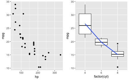
So, grid.arrange is the key.

Plots from png-file

comb2pngs <- function(imgs, bottom_text = NULL){
  img1 <-  grid::rasterGrob(as.raster(readPNG(imgs[1])),
                            interpolate = FALSE)
  img2 <-  grid::rasterGrob(as.raster(readPNG(imgs[2])),
                            interpolate = FALSE)
  grid.arrange(img1, img2, ncol = 2, bottom = bottom_text)
}

The code of this function was inspired by code from Ben from this SO post.

Now, let’s load two pngs and then call the function above.

png1_path <- "https://sebastiansauer.github.io/images/2016-08-30-03.png"
png2_path <- "https://sebastiansauer.github.io/images/2016-08-31-01.png"


png1_dest <- "https://sebastiansauer.github.io/images/2017-10-12/img1.png"
png2_dest <- "https://sebastiansauer.github.io/images/2017-10-12/img2.png"


#download(png1_path, destfile = png1_dest)
#download(png2_path, destfile = png2_dest)

comb2pngs(c(png1_dest, png2_dest))

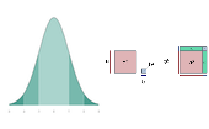
This works, it produces two plots from png files side by side.

Two plots side-by-side the knitr way. Does not work.

But what about the standard knitr way?

knitr::include_graphics(c(png1_dest,png2_dest))

<img src=”“https://sebastiansauer.github.io/images/2017-10-12/img1.png” title=”plot of chunk unnamed-chunk-4” alt=”plot of chunk unnamed-chunk-4” width=”30%” style=”display: block; margin: auto;” /><img src=”“https://sebastiansauer.github.io/images/2017-10-12/img2.png” title=”plot of chunk unnamed-chunk-4” alt=”plot of chunk unnamed-chunk-4” width=”30%” style=”display: block; margin: auto;” />

Does not work.

Maybe with only one value for out.width??

knitr::include_graphics(c(png1_dest, png2_dest))

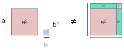
Nope. Does not work.

Does not work either, despite some saying so.

Maybe two times include_graphics?

imgs <- c(png1_dest, png2_dest)
imgs
#> [1] "https://sebastiansauer.github.io/images/2017-10-12/img1.png"
#> [2] "https://sebastiansauer.github.io/images/2017-10-12/img2.png"

knitr::include_graphics(png1_dest);  knitr::include_graphics(png2_dest)

An insight why include_graphics fails

No avail. Looking at the html code in the md-file which is produced by the knitr -call shows one interesting point: all this version of include_graphics produce the same code. And all have this style="display: block; margin: auto;" part in it. That obviously created problems. I am unsure who to convince include_graphics to divorce from this argument. I tried some versions of the chunk argument fig.show = hold, but to no avail.

Plain markdown works

Try this code ![](https://sebastiansauer.github.io/images/2017-10-12/img1.png){ width=30% } ![](https://sebastiansauer.github.io/images/2017-10-12/img2.png){ width=40% } The two commands ![]... need not appear in one row. However, no new paragraph may separate them (no blank line between, otherwise the images will appear one below the other).

{ width=30% } { width=40% }

Works. But the markdown way does not give the fill comfort and power. So, that’s not quite perfect.

Conclusion

A partial solution is there; but it’s not optimal. There wil most probably be different alternatives. For example, using plain html or Latex. But it’s a kind of pity, the include_graphics call does not work as expected (by me).