There is the idea that the alt-right German party AfD is followed by those who are deprived of chances, thoses of fearing to falling down the social ladder, and so on. Let’s test this hypothesis. No, I am not thinking on hypothesis testing, p-values, and stuff. Rather, let’s color a map of German election districts (Wahlkreise) according to whether the area is poor AND the AfD gained a lot of votes (and vice versa: the area is rich AND the AfD gained relatively few votes). More specifically, let’s look at unemployment ratios and incomes at different election areas in the country and compare those figures to AfD election results.
In a similar vein, one could put forward the “unemployment-AfD-accordance hypothesis”: The rank order of a given area is equal (or similar) to the AfD vote rank order. Let’s test this hypothesis in this post.
Packages
library(sf)
library(stringr)
library(tidyverse)
library(readxl)
library(magrittr)
library(huxtable)
library(broom)
Geo data
In this post, we try to map election areas of Germany (“Wahlkreise”) to three types of statistical data:
- AfD election results
- unemployment ratio and/or
- income
:attention: The election ratios are unequal to the district areas (as far as I know, not complete identical to the very least). So will need to get some special geo data. This geo data is available here and the others links on that page.
Download and unzip the data; store them in an appropriate folder. Adjust the path to your needs:
my_path_wahlkreise <- "~/Documents/datasets/geo_maps/btw17_geometrie_wahlkreise_shp/Geometrie_Wahlkreise_19DBT.shp"
file.exists(my_path_wahlkreise)
## [1] TRUE
wahlkreise_shp <- st_read(my_path_wahlkreise)
## Reading layer `Geometrie_Wahlkreise_19DBT' from data source `/Users/sebastiansauer/Documents/datasets/geo_maps/btw17_geometrie_wahlkreise_shp/Geometrie_Wahlkreise_19DBT.shp' using driver `ESRI Shapefile'
## Simple feature collection with 299 features and 4 fields
## geometry type:  MULTIPOLYGON
## dimension:      XY
## bbox:           xmin: 280387.7 ymin: 5235855 xmax: 921025.5 ymax: 6101444
## epsg (SRID):    NA
## proj4string:    +proj=utm +zone=32 +ellps=GRS80 +units=m +no_defs
glimpse(wahlkreise_shp)
## Observations: 299
## Variables: 5
## $ WKR_NR    <int> 1, 2, 3, 4, 5, 6, 7, 8, 9, 10, 11, 12, 13, 14, 15, 1...
## $ LAND_NR   <fctr> 01, 01, 01, 01, 01, 01, 01, 01, 01, 01, 01, 13, 13,...
## $ LAND_NAME <fctr> Schleswig-Holstein, Schleswig-Holstein, Schleswig-H...
## $ WKR_NAME  <fctr> Flensburg – Schleswig, Nordfriesland – Dithmarschen...
## $ geometry  <simple_feature> MULTIPOLYGON (((543474.9057..., MULTIPOLY...
wahlkreise_shp %>%
  ggplot() +
  geom_sf()
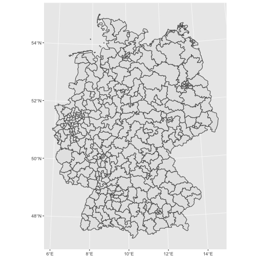
That was easy, right? The sf package fits nicely with the tidyverse. Hence not much to learn in that regard. I am not saying that geo data is simple, quite the contrary. But luckily the R functions fit in a well known schema.
For instance, let’s remove the axis labels and let’s fill the country with some different color. Hm, what’s the color of Germany? Grey? Black (color of the leading party)? Black-red-gold?
wahlkreise_shp %>%
  ggplot() +
  geom_sf(fill = "grey40") +
  theme_void()
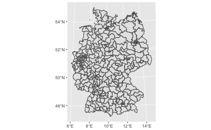
Ok, that’s complete. How many of those “WahlKreise” do we have? 318, it appears. At least (that’s the number of rows in the dataframe). That’s not exactly the number of administrative districts in Germany, which is 401.
unemployment ratios
These data can as well be fetched from the same site as above, as mentioned above, we need to make sure that we have the statistics according to the election aras, not the administrative areas.
unemp_file <- "~/Documents/datasets/Strukturdaten_De/btw17_Strukturdaten-utf8.csv"

file.exists(unemp_file)
## [1] TRUE
unemp_de_raw <- read_delim(unemp_file,
    ";", escape_double = FALSE,
    locale = locale(decimal_mark = ",",
        grouping_mark = "."),
    trim_ws = TRUE,
    skip = 8)  # skipt the first 8 rows
## Parsed with column specification:
## cols(
##   .default = col_double(),
##   Land = col_character(),
##   `Wahlkreis-Nr.` = col_integer(),
##   `Wahlkreis-Name` = col_character(),
##   `Gemeinden am 31.12.2015 (Anzahl)` = col_integer(),
##   `Verfügbares Einkommen der privaten Haushalte 2014 (€ je Einwohner)` = col_integer(),
##   `Bruttoinlandsprodukt 2014 (€ je Einwohner)` = col_integer(),
##   `Absolventen/Abgänger beruflicher Schulen 2015` = col_character(),
##   `Sozialversicherungspflichtig Beschäftigte am 30.06.2016 - Land- und Forstwirtschaft, Fischerei (%)` = col_character(),
##   `Sozialversicherungspflichtig Beschäftigte am 30.06.2016 - Produzierendes Gewerbe (%)` = col_character(),
##   `Sozialversicherungspflichtig Beschäftigte am 30.06.2016 - Handel, Gastgewerbe, Verkehr (%)` = col_character(),
##   `Sozialversicherungspflichtig Beschäftigte am 30.06.2016 - Öffentliche und private Dienstl eister (%)` = col_character(),
##   Fußnoten = col_character()
## )
## See spec(...) for full column specifications.
#glimpse(unemp_de_raw)
Jezz, we need to do some cleansing before we can work with this dataset.
unemp_names <- names(unemp_de_raw)

unemp_de <- unemp_de_raw

names(unemp_de) <- paste0("V",1:ncol(unemp_de))
The important columns are:
unemp_de <- unemp_de %>%
rename(state = V1,
area_nr = V2,
area_name = V3,
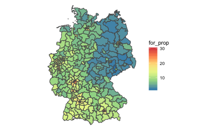
for_prop = V8,
pop_move = V11,
pop_migr_background = V19,
income = V26,
unemp = V47) # total, as to March 2017
AfD election results
Again, we can access the data from the same source, the Bundeswahlleiter here. I have prepared the column names of the data and the data structure, to render the file more accessible to machine parsing. Data points were not altered. You can access my version of the file here.
elec_file <- "~/Documents/datasets/Strukturdaten_De/btw17_election_results.csv"
file.exists(elec_file)
## [1] TRUE
elec_results <- read_csv(elec_file)
## Parsed with column specification:
## cols(
##   .default = col_integer(),
##   Gebiet = col_character(),
##   Waehler_Erststimmen_vorlaeufig = col_double(),
##   Waehler_Zweitsimmen_vorlaeufig = col_double(),
##   Waehler_ungueltige_Zweitstimmen_vorlauefig = col_double(),
##   CDU_Erststimmen_Vorperiode = col_character(),
##   CDU_Zweitstimmen_Vorperiode = col_double(),
##   Gruene3 = col_double(),
##   Gruene4 = col_double(),
##   AfD3 = col_double(),
##   AfD4 = col_double(),
##   Piraten4 = col_double(),
##   Vorperiode__3 = col_double(),
##   Vorläufig__4 = col_double(),
##   Vorperiode__18 = col_character(),
##   Vorperiode__20 = col_character(),
##   Vorläufig__22 = col_character(),
##   Vorperiode__22 = col_character(),
##   Vorperiode__23 = col_character(),
##   Vorperiode__24 = col_character(),
##   Vorperiode__25 = col_character()
##   # ... with 46 more columns
## )
## See spec(...) for full column specifications.
For each party, four values are reported:
- primary vote, present election
- primary vote, previous election
- secondary vote, present election
- secondary vote, previous election
The secondary vote refers to the party, that’s what we are interested in (column 46). The primary vote refers to the candidate of that area; the pimary vote may also be of similar interest, but that’s a slightly different question, as it taps more into the approval of a person, rather to a party (of course there’s a lot overlap between both in this situation).
# names(elec_results)
afd_prop <- elec_results %>%
  select(1, 2, 46, 18) %>%
  rename(afd_votes = AfD3,
         area_nr = Nr,
         area_name = Gebiet,
         votes_total = Waehler_gueltige_Zweitstimmen_vorlauefig) %>%
  mutate(afd_prop = afd_votes / votes_total) %>%
  na.omit
In the previous step, we have selected the columns of interest, changed their name (shorter, English), and have computed the proportion of (valid) secondary votes in favor of the AfD.
Match unemployment and income to AfD votes for each Wahlkreis
wahlkreise_shp %>%
  left_join(unemp_de, by = c("WKR_NR" = "area_nr")) %>%
  left_join(afd_prop, by = "area_name") -> chloro_data
Plot geo map with afd votes
chloro_data %>%
  ggplot() +
  geom_sf(aes(fill = afd_prop)) -> p1
p1
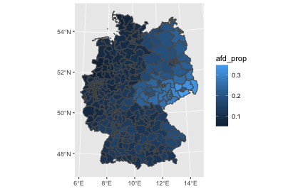
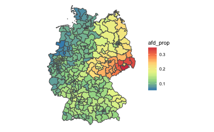
We might want to play with the fill color, or clean up the map (remove axis etc.)
p1 + scale_fill_distiller(palette = "Spectral") +
  theme_void()
Geo map (of election areas) with unemployment map
chloro_data %>%
  ggplot() +
  geom_sf(aes(fill = unemp)) +
  scale_fill_distiller(palette = "Spectral") +
  theme_void() -> p2
p2
Concordance of AfD results and unemployment/income
Let’s compute the percent ranking for each of the variables of interest (AfD votes, unemployment ratio, and income). Then we can compute the concordance for each pair by simply computing the difference (or maybe absolute difference). After that, we plot this “concordance variables” as fill color to the map.
chloro_data %>%
  mutate(afd_rank = percent_rank(afd_prop),
         unemp_rank = percent_rank(unemp),
         income_rank = percent_rank(income)) %>%
  mutate(afd_income_diff = subtract(afd_rank, income_rank),
         afd_unemp_diff = subtract(afd_rank, unemp_rank)) -> chloro_data
Let’s check the first ranks for each of the variables of interest. AfD ranks first:
chloro_data %>%
  as.data.frame %>%
  select(area_name, afd_rank, afd_prop, unemp_rank, income_rank) %>%
  arrange(-afd_rank) %>%
  slice(1:5)
## # A tibble: 5 x 5
##                          area_name  afd_rank  afd_prop unemp_rank
##                              <chr>     <dbl>     <dbl>      <dbl>
## 1 Sächsische Schweiz-Osterzgebirge 1.0000000 0.3546391  0.5637584
## 2                          Görlitz 0.9966443 0.3288791  0.9463087
## 3                           Meißen 0.9932886 0.3287724  0.7114094
## 4                        Bautzen I 0.9899329 0.3276397  0.6476510
## 5                    Mittelsachsen 0.9865772 0.3124584  0.5872483
## # ... with 1 more variables: income_rank <dbl>
Saxonia leads. Unemployment “top” places:
chloro_data %>%
  as.data.frame %>%
  select(area_name, afd_prop, unemp_rank, income_rank) %>%
  arrange(-unemp_rank) %>%
  slice(1:5)
## # A tibble: 5 x 4
##                                    area_name  afd_prop unemp_rank
##                                        <chr>     <dbl>      <dbl>
## 1                              Gelsenkirchen 0.1703539  1.0000000
## 2                                 Duisburg I 0.1132661  0.9932886
## 3                                Duisburg II 0.1542772  0.9932886
## 4 Vorpommern-Rügen – Vorpommern-Greifswald I 0.1964088  0.9832215
## 5                                   Essen II 0.1496040  0.9832215
## # ... with 1 more variables: income_rank <dbl>
The Ruhrpott is ahead of this sad pack. And the lowest unemployment ranks are at:
chloro_data %>%
  as.data.frame %>%
  select(area_name, afd_prop, unemp_rank, income_rank) %>%
  arrange(unemp_rank) %>%
  slice(1:5)
## # A tibble: 5 x 4
##            area_name  afd_prop  unemp_rank income_rank
##                <chr>     <dbl>       <dbl>       <dbl>
## 1 Erding – Ebersberg 0.1191024 0.000000000   0.9496644
## 2           Freising 0.1356325 0.003355705   0.7751678
## 3         Donau-Ries 0.1470312 0.003355705   0.8255034
## 4         Ingolstadt 0.1513400 0.010067114   0.5973154
## 5            Neu-Ulm 0.1511712 0.010067114   0.8456376
And finale income, low 5 and top 5:
chloro_data %>%
  as.data.frame %>%
  select(area_name, afd_prop, unemp_rank, income_rank) %>%
  arrange(income_rank) %>%
  slice(c(1:5, 294:299))
## # A tibble: 11 x 4
##                             area_name   afd_prop unemp_rank income_rank
##                                 <chr>      <dbl>      <dbl>       <dbl>
##  1                      Gelsenkirchen 0.17035387 1.00000000 0.000000000
##  2                          Leipzig I 0.20813820 0.79530201 0.003355705
##  3                         Leipzig II 0.15977744 0.79530201 0.003355705
##  4                              Halle 0.17787876 0.92281879 0.010067114
##  5                         Duisburg I 0.11326607 0.99328859 0.013422819
##  6 Bad Tölz-Wolfratshausen – Miesbach 0.11688174 0.04026846 0.983221477
##  7                        Main-Taunus 0.10320408 0.20805369 0.986577181
##  8                         Hochtaunus 0.11155599 0.23825503 0.989932886
##  9      Starnberg – Landsberg am Lech 0.09900204 0.04026846 0.993288591
## 10                          Heilbronn 0.16416233 0.26174497 0.996644295
## 11                       München-Land 0.09399476 0.03355705 1.000000000
Now plot.
chloro_data %>%
  ggplot() +
  geom_sf(aes(fill = afd_unemp_diff)) +
  scale_fill_gradient2() +
  theme_void() -> p3
p3
The fill color denotes the difference between unemployment rank of a given area and its afd vote rank. For example, if area X has an unemployment rank of .5 (50%), it means that half of the areas in the country have a lower (higher) unemployment ratio, respectively (the median). Similarly, an AfD vote rank of .5 indicates the median position. The difference of these two figures is zero, indicating accordance or close match. Thus, figures around zero denote accordance or match. 1 (100%) of AfD vote rank indicates the area with the best AfD results (area with the most votes); similar reasoning applies for income and unemployment ratio.
Hence, numbers greater than zero indicate that the AfD scored better than it would be expected by the accordance-hypothesis.
Similarly, numbers smaller than zero indicate that the AfD scored better than it would be expected by the accordance-hypothesis.
Areas with (near) white filling provide some support for the accordance hypothesis. There are areas of this type, but it is not the majority. The vast majority of areas showed too much or too little AfD - relative to their unemployment ratio.
This reasonsing shows that the AfD received better results in southern and middle areas of Germany than it would be expected by the accordance hypothesis. In contrast, the more poorer northern areas voted for the AfD much less often than it would be expected by the accordance hypothesis.
Let’s look at the areas with minimal and maximal dis-accordance, out of curiosity.
chloro_data %>%
  as.data.frame %>%
  select(area_name, afd_unemp_diff, unemp, afd_prop) %>%
  arrange(afd_unemp_diff) %>%
  slice(c(1:5, 295:299)) %>% hux %>%
  add_colnames
| area_name | afd_unemp_diff | unemp | afd_prop |
| Essen III | -0.85 | 11.90 | 0.08 |
| Berlin-Friedrichshain-Kreuzberg – Prenzlauer Berg Ost | -0.83 | 9.40 | 0.06 |
| Köln II | -0.80 | 8.50 | 0.05 |
| Kiel | -0.78 | 8.80 | 0.07 |
| Bremen I | -0.77 | 9.80 | 0.08 |
| Deggendorf | 0.71 | 3.60 | 0.19 |
| Rottal-Inn | 0.76 | 3.10 | 0.17 |
| Donau-Ries | 0.77 | 2.20 | 0.15 |
| Neu-Ulm | 0.78 | 2.50 | 0.15 |
| Ingolstadt | 0.78 | 2.50 | 0.15 |
And areas with high accordance (diff score close to zero):
chloro_data %>%
  as.data.frame %>%
  select(area_name, afd_unemp_diff, unemp, afd_prop) %>%
  arrange(afd_unemp_diff) %>%
  filter(afd_unemp_diff > -0.05, afd_unemp_diff < .05) %>%
  hux %>%
  add_colnames
| area_name | afd_unemp_diff | unemp | afd_prop |
| Rostock – Landkreis Rostock II | -0.04 | 8.90 | 0.16 |
| Offenbach | -0.03 | 6.60 | 0.12 |
| Berlin-Lichtenberg | -0.03 | 9.40 | 0.17 |
| Rhein-Sieg-Kreis I | -0.03 | 5.20 | 0.10 |
| Mosel/Rhein-Hunsrück | -0.03 | 4.10 | 0.09 |
| Berlin-Treptow-Köpenick | -0.02 | 9.40 | 0.17 |
| Herzogtum Lauenburg – Stormarn-Süd | -0.02 | 4.80 | 0.10 |
| Helmstedt – Wolfsburg | -0.01 | 5.80 | 0.11 |
| Oberbergischer Kreis | -0.01 | 5.50 | 0.11 |
| Kreuznach | -0.01 | 6.40 | 0.12 |
| Herford – Minden-Lübbecke II | -0.01 | 5.70 | 0.11 |
| Mansfeld | -0.01 | 10.20 | 0.24 |
| Siegen-Wittgenstein | 0.00 | 5.40 | 0.11 |
| Minden-Lübbecke I | 0.01 | 5.30 | 0.11 |
| Heidelberg | 0.01 | 4.30 | 0.09 |
| Leipzig II | 0.01 | 8.30 | 0.16 |
| Neuwied | 0.02 | 5.30 | 0.11 |
| Osterholz – Verden | 0.03 | 4.40 | 0.10 |
| Prignitz – Ostprignitz-Ruppin – Havelland I | 0.03 | 8.90 | 0.19 |
| Dessau – Wittenberg | 0.04 | 9.10 | 0.20 |
| Elbe-Elster – Oberspreewald-Lausitz II | 0.04 | 9.60 | 0.25 |
Similar story for income.
chloro_data %>%
  ggplot() +
  geom_sf(aes(fill = afd_income_diff)) +
  scale_fill_gradient2() +
  theme_void() -> p4
p4
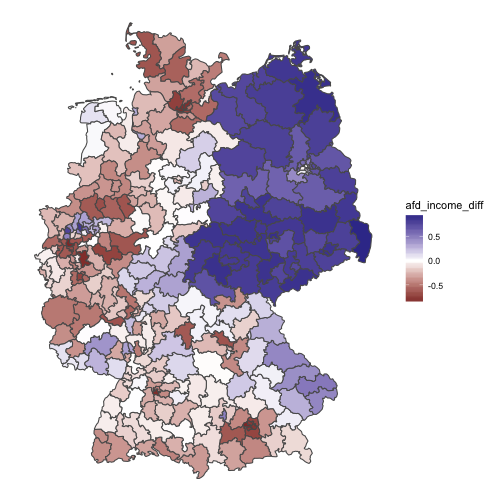
The map shows a clear pattern: The eastern parts of Germany are far more afd-oriented than their income rank would predict (diff scores above zero, blue color). However, for some areas across the whole rest of the country, the likewise pattern is true too: A lot areas are rich and do not vote for the AfD (reddish color, diff score below zero). And, thirdly, a lot of aras support the accordance hypothesis (white color, diff score around zero).
More simple map
Maybe we should simplify the map: Let’s only distinguish three type of areas: too much AfD in comparison to the unemployment, too few AfD for the unemployment, or AfD at par with unemployment. Maybe the picture is more clearcut then.
chloro_data %>%
  select(afd_unemp_diff) %>%
  mutate(afd_unemp_diff_3g = cut_interval(afd_unemp_diff, n = 3,
         labels = c("AFD < Arbeitslosigkeit",
                    "AFD = Arbeitslosigkeit",
                    "AFD > Arbeitslosigkeit"))) %>%
  ggplot() +
  geom_sf(aes(fill = afd_unemp_diff_3g)) +
  labs(fill) +
  theme_void()
“AfD density”
In a similar vein, we could compute the ratio of AfD votes and unemployment. That would give us some measure of covariability. Let’s see.
library(viridis)
chloro_data %>%
  mutate(afd_dens = afd_prop / unemp) %>%
  ggplot +
  geom_sf(aes(fill = afd_dens)) +
  theme_void() +
  scale_fill_viridis()
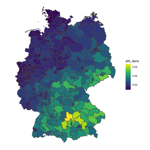
The diagram shows that in relation to unemployment, the AfD votes are strongest in central Bavaria (Oberbayern). Don’t forget that this measure is an indication of co-occurence, not of absolute AfD votes.
Correlation of unemployment and AfD votes
A simple, straight-forward and well-known approach to devise assocation strength is Pearson’s correlation coefficient. Oldie but goldie. Let’s depict it.
chloro_data %>%
  select(unemp, afd_prop, income, area_name) %>%
  ggplot +
  aes(x = unemp, y = afd_prop) +
  geom_point() +
  geom_smooth()
## `geom_smooth()` using method = 'loess' and formula 'y ~ x'
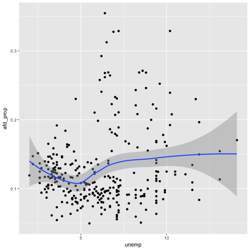
The correlation itself is
chloro_data %>%
  select(unemp, afd_prop, income, area_name) %>%
  as.data.frame %T>%
  summarise(cor_afd_unemp = cor(afd_prop, unemp)) %>%
  do(tidy(cor.test(.$afd_prop, .$unemp)))
##    estimate statistic     p.value parameter  conf.low conf.high
## 1 0.1834224    3.2156 0.001445273       297 0.0714793 0.2908024
##                                 method alternative
## 1 Pearson's product-moment correlation   two.sided
Which is not strong, but is certainly more than mere noise (and p-value below some magic number).
Regression residuals of predicting unemployment by afd_score
Let’s predict the AfD vote score taking the unemployment as an predictor. Then let’s plot the residuals to see how good the prediction is, ie., how close (or rather, far) the association of unemployment and AfD voting is.
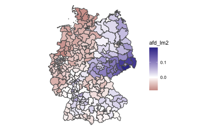
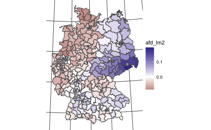
lm1 <- lm(afd_prop ~ unemp, data = chloro_data)

chloro_data %>%
  mutate(afd_lm1 = lm(afd_prop ~ unemp, data = .)$residuals) -> chloro_data
And now plot the residuals:
chloro_data %>%
  select(afd_lm1) %>%
  ggplot() +
  geom_sf(aes(fill = afd_lm1)) +
  scale_fill_gradient2() +
  theme_void()
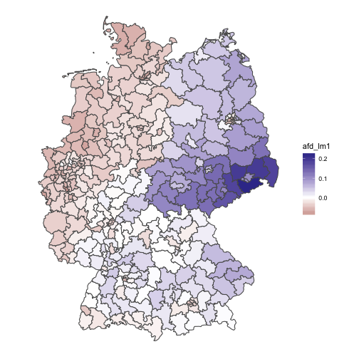
Interesting! This model shows a clearcut picture: The eastern part is too “afd” for its unemployment ratio (some parts of east-southern Bavaria too); the west is less afd-ic than what would be expected by the unemployment. The rest (middle and south) parts over-and-above show the AfD levels that woul be expected by their unemployment.
Conclusion
The regression model provides a quite clearcut picture, much more than the rank difference has unveiled. The difference in information may be due to the fact that the rank difference is of ordinal level only, and hence omits information compared to the regression level. The story of the data may thus be summarized in easy words: The higher the unemployment ratio, the higher the AfD ratio. However, this is only part of the story. unemployment explains a rather small fraction of AfD votes. Yet, given the multitude of potential influences on voting behavior, a correlation coefficient of .18 is not negligible, rather substantial.