Let’s get purrr. Recently, I ran across this issue: A data frame with many columns; I wanted to select all numeric columns and submit them to a t-test with some grouping variables.
As this is a quite common task, and the purrr-approach (package purrr by @HadleyWickham) is quite elegant, I present the approach in this post.
Let’s load the data, the Affairs data set, and some packages:
data(Affairs, package = "AER")
library(purrr)  # functional programming
library(dplyr)  # dataframe wrangling
library(ggplot2)  # plotting
library(tidyr)  # reshaping df
Don’t forget that the four packages need to be installed in the first place.
So, now let’s select all numeric variables from the data set. dplyr and purrr provide functions for that purpose, very convenient:
Affairs %>%
select_if(is.numeric) %>% head
##    affairs age yearsmarried religiousness education occupation rating
## 4        0  37        10.00             3        18          7      4
## 5        0  27         4.00             4        14          6      4
## 11       0  32        15.00             1        12          1      4
## 16       0  57        15.00             5        18          6      5
## 23       0  22         0.75             2        17          6      3
## 29       0  32         1.50             2        17          5      5
In the next step, we “map” each of these columns to a function, here the t-test.
Affairs %>%
  select_if(is.numeric) %>%
  map(~t.test(. ~ Affairs$gender)$p.value)
## $affairs
## [1] 0.7739606
##
## $age
## [1] 2.848452e-06
##
## $yearsmarried
## [1] 0.458246
##
## $religiousness
## [1] 0.8513998
##
## $education
## [1] 9.772643e-24
##
## $occupation
## [1] 8.887471e-35
##
## $rating
## [1] 0.8533625
the map function may look obscure if you have not seen it before. As said, the map function maps each column to the function you mention. The ~t.test() bit means that you define an anonymous function, just as you would for normal apply calls, for example. So equivalently, one could write:
Affairs %>%
  select_if(is.numeric) %>%
  #map(~t.test(. ~ Affairs$gender)$p.value) %>%
  map(function(x) t.test(x ~ Affairs$gender)$p.value)
## $affairs
## [1] 0.7739606
##
## $age
## [1] 2.848452e-06
##
## $yearsmarried
## [1] 0.458246
##
## $religiousness
## [1] 0.8513998
##
## $education
## [1] 9.772643e-24
##
## $occupation
## [1] 8.887471e-35
##
## $rating
## [1] 0.8533625
The ~ is just a convenient short hand for the normal way of writing anonymous functions. And the dot . is then again a shorthand for the column that is handed through the function (just as xin the normal apply call).
Well, that’s basically it! The $p.value bit just extracts the p-value statistic out of the t-test object.
The more familiar, lapply approach would be something like:
lapply(Affairs[c("affairs", "age", "yearsmarried")], function(x) t.test(x ~ Affairs$gender))
## $affairs
##
## 	Welch Two Sample t-test
##
## data:  x by Affairs$gender
## t = -0.28733, df = 594.01, p-value = 0.774
## alternative hypothesis: true difference in means is not equal to 0
## 95 percent confidence interval:
##  -0.6068861  0.4519744
## sample estimates:
## mean in group female   mean in group male
##             1.419048             1.496503
##
##
## $age
##
## 	Welch Two Sample t-test
##
## data:  x by Affairs$gender
## t = -4.7285, df = 575.26, p-value = 2.848e-06
## alternative hypothesis: true difference in means is not equal to 0
## 95 percent confidence interval:
##  -5.014417 -2.071219
## sample estimates:
## mean in group female   mean in group male
##             30.80159             34.34441
##
##
## $yearsmarried
##
## 	Welch Two Sample t-test
##
## data:  x by Affairs$gender
## t = -0.74222, df = 595.53, p-value = 0.4582
## alternative hypothesis: true difference in means is not equal to 0
## 95 percent confidence interval:
##  -1.2306829  0.5556058
## sample estimates:
## mean in group female   mean in group male
##             8.017070             8.354608
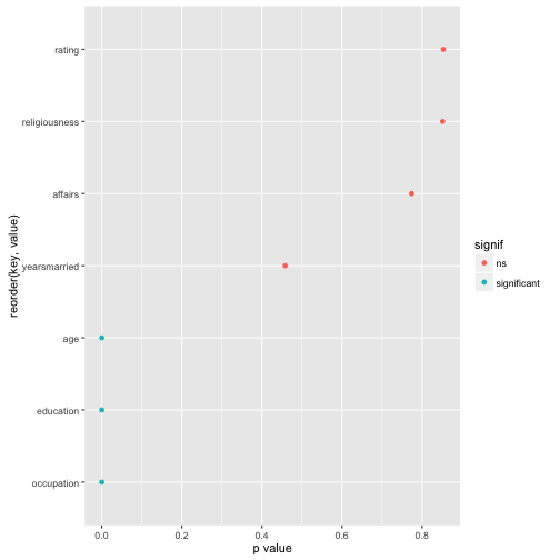
Now, finally, let’s plot the result for easier comprehension. Some minor wrangling of the data is necessary:
Affairs %>%
  select_if(is.numeric) %>%
  #na.omit() %>%
  map(~t.test(. ~ Affairs$gender)$p.value) %>%
  as.data.frame %>%
  gather %>%
  mutate(signif = ifelse(value < .05, "significant", "ns")) %>%
  ggplot(aes(x = reorder(key, value), y = value)) +
  geom_point(aes(color = signif)) +
  coord_flip() +
  ylab("p value")
