The logistic regression is an incredible useful tool, partly because binary outcomes are so frequent in live (“she loves me - she doesn’t love me”). In parts because we can make use of well-known “normal” regression instruments.

But the formula of logistic regression appears opaque to many (beginners or those with not so much math background).

Let’s try to shed some light on the formula by discussing some accessible explanation on how to derive the formula.

Plotting the logistics curve

Let’s have a look at the curve of the logistic regression.

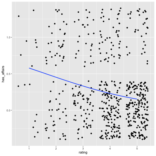
For example, let’s look at the question of whether having extramarital affairs is a function of marital satisfaction.

library(tidyverse)
data(Affairs, package = "AER")

Affairs$has_affairs <- if_else(condition = Affairs$affairs > 0, 1, 0)

Affairs %>% 
  ggplot() +
  aes(x = rating,y = has_affairs) +
  geom_jitter() +
  geom_smooth(aes(y = has_affairs), method = "glm", method.args = list(family = "binomial"), se = FALSE)

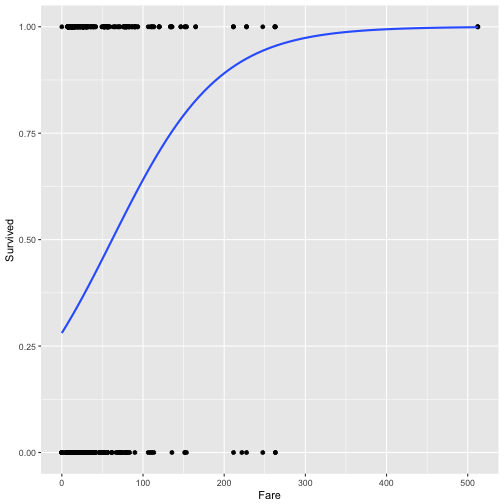
Hm, the curve does not pop out to vividly. Let’s have a look at some other data, why not the Titanic disaster data. Can the survival chance plausible put as a function of the cabin fare?

data(titanic_train, package = "titanic")

titanic_train %>% 
  ggplot() +
  aes(x = Fare,y = Survived) +
  geom_point() +
  geom_smooth(aes(y = Survived), method = "glm", method.args = list(family = "binomial"), se = FALSE)

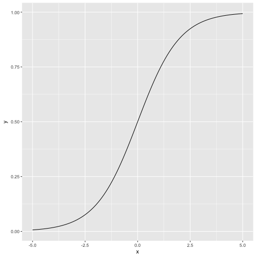
Hm, maybe better to look at the curve in general.

logist <- function(x){
  y = exp(x) / (1 + exp(x))
}

p1 <- ggplot(data_frame())

p1 + stat_function(aes(-5:5), fun = logist) + xlab("x")

Ok, better.

Functional form

It is well-known that the fucntional form of the logictic regression curve is

where \(e\) is Euler’s number (2.718…) and \(t\) can be any linear combination of predictors such as \(b0 + b1x\). \(Y=1\) indicates that the event in question has occured (eg., “survived”, “has_affairs”).

Assume that \(t\) is \(b0 + b1x\) then

Now what? Well, we would to end up with the “typical” formula of the logistic regression, something like:

where \(L\) is the Logit, i.e.,

Deriving the formula

Ok, in a first step, let’s take our \(p(Y=1) = f(t)\) and divide by the probability of the complementary event. If the probability of event \(A\) is \(p\), the the probability of \(not-A\) is \(1-p\). Thus

So wat did we do? We have just replaced \(f(t)\) by \(\frac{e^t}{1e^t}\), and have therey computed the odds.

Next, we multiply the equation by \(\frac{1+e^t}{1+e^t}\) (which is the neutral element, 1), yielding.

In other words, the denominator of the numerator “wandered” down to the denominator.

Now, we can simplify the denominator a bit:

Simplifying the denominator further

But the denominator simplifies to $1$, as can be seen here

so the final solution is

\(=e^t\).

Ok, great, but what does this solution tells us? It tells us the that the odds simplify to \(e^t\).

Now, let’s take the (natural) logarithm of this expression.

by the rules of exponents algebra.

But \(t = b0 + b1x\).

In sum

The left part of the previous equation is called the logit which is “odds plus logarithm” of \(f(t)\), or rather, more precisely, the logarithm of the odss of \(p/(1-p)\).

Looking back, what have we gained? We now know that if we take the logit of any linear combination, we will get the logistic regression formula. In simple words: “Take the normal regression equation, apply the logit \(L\), and you’ll get out the logistic regression” (provided the criterion is binary).

\(L(t) = ln\left( \frac{f(t)}{1-f(t)}\right) = b0 + b1x\).

The formula of the logistic regression is similar in the “normal” regression. The only difference is that the logit function has been applied to the “normal” regression formula.

The linearity of the logit helps us to apply our standard regression vocabulary: “If X is increased by 1 unit, the logit of Y changes by b1”. Just insert “the logit”; the rest of the sentence is the normal regression parlance.

Note that the slope of the curve is not linear, hence b1 is not equal for all values of X.