Correlation is one of the most widely used and a well-known measure of the assocation (linear association, that is) of two variables.

Perhaps less well-known is that the correlation is in principle identical to the covariation.

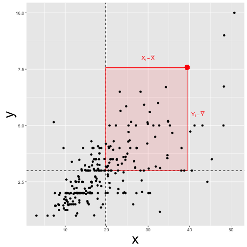
To see this, consider the a formula of the covariance of two empirical datasets, \(X\) and \(Y\):

In other words, the covariance of $X$ and $Y$ $COV(X,Y)$ is the average of difference of some value to its mean.

This idea is conveyed by this picture:

The covariance is identical to the correlation (?)

What does it mean to say the (coefficient of) correlation is “identical” to the covariation?

If we “feed” z-scaled values to the covariation, we will get back the correlation.

In other words, the correlation equals the covariation if the data are z-scaled.

So, let’s see. We replace \(X\) by \(z_X\) and \(Y\) by \(z_Y\) and see what happens.

However, \(z_{\bar{X}} = 0\), and by analogy, \(z_{\bar{y}} = 0\). So the eqaution simplifies to

Now, \(z_x\) can be expressed as

The same rule applies for \(z_y\), by analogy.

Now, let’s insert the previous equation in the equation of \(Cov(z_X, z_Y)\):

\(sd_X$ and $sd_Y\) can be pulled out of the sum, right at the front of the equation, leaving us with

\(Cov(z_X, z_Y) = \frac{1}{sd_X \cdot sd_Y} \cdot \big( \sum (X_i - \bar{X}) \cdot (Y_i - \bar{Y}) \big)\).

And that’s the definition of the correlation of \(X\) and \(Y\), more frequently put this way:

\(Cov(z_X, z_Y) = \frac {\sum (X_i - \bar{X}) \cdot (Y_i - \bar{Y})}{sd_X \cdot sd_Y}\).

Hence,

\(Cov(z_X, z_Y) = cor(X,Y)\).

Example time

It is helpful to consider an example.

This is a scatterplot of two variables, ie., “raw data” as is “fed in” for the calculation of the (empirical) covariation:

library(tidyverse)
mtcars %>% 
  ggplot +
  aes(x = hp, y = mpg) +
  geom_point()

And now, let’s z-scale the two variables and draw the same diagram again:

mtcars %>% 
  select(hp, mpg) %>% 
  mutate_all(funs(scale)) %>% 
  ggplot +
  aes(x = hp, y = mpg) +
  geom_point()

Now, what’s the difference? Nada, no difference. That’s reassuring, because we just derived that the assocation of the variables is the same - no matter if use the raw data or z-scaled data as input. The diagrams confirms this in an more intuitive way.

Summary

The correlation is a “special case” of the covariance; it is the case when we feed z-scaled data to the covariance.

Happy data analyzing!