Logistic regression may give a headache initially. While the structure and idea is the same as “normal” regression, the interpretation of the b’s (ie., the regression coefficients) can be more challenging.
This post provides a convenience function for converting the output of the glm function to a probability. Or more generally, to convert logits (that’s what spit out by glm) to a probabilty.
Note1: The objective of this post is to explain the mechanics of logits. There are more convenient tools out there. (Thanks to Jack’s comment who made me adding this note.)
Note2: I have corrected an error pointed out by Jana’s comment, below (you can always check older versions on the Github repo).
Example time
So, let’s look at an example. First load some data (package need be installed!):
data(titanic_train, package = "titanic")
d <- titanic_train  # less typing
Compute a simple glm:
glm1 <- glm(Survived ~ Pclass, data = d, family = "binomial")
The coeffients are the interesting thing:
coef(glm1)
## (Intercept)      Pclass
##   1.4467895  -0.8501067
These coefficients are in a form called ‘logits’.
Takeaway
If coefficient (logit) is positive, the effect of this predictor (on survival rate) is positive and vice versa.
Here Pclass coefficient is negative indicating that the higher Pclass the lower is the probability of survival.
Conversion rule
To convert a logit (glm output) to probability, follow these 3 steps:
- Take
glmoutput coefficient (logit) - compute e-function on the logit using
exp()“de-logarithimize” (you’ll get odds then) - convert odds to probability using this formula
prob = odds / (1 + odds). For example, sayodds = 2/1, then probability is2 / (1+2)= 2 / 3(~.67)
R function to rule ‘em all (ahem, to convert logits to probability)
This function converts logits to probability.
logit2prob <- function(logit){
  odds <- exp(logit)
  prob <- odds / (1 + odds)
  return(prob)
}
For convenience, you can source the function like this:
source("https://sebastiansauer.github.io/Rcode/logit2prob.R")
For our glm:
logit2prob(coef(glm1))
## (Intercept)      Pclass
##   0.8095038   0.2994105
How to convert logits to probability
How to interpret:
- The survival probability is 0.8095038 if
Pclasswere zero (intercept). - However, you cannot just add the probability of, say
Pclass == 1to survival probability ofPClass == 0to get the survival chance of 1st class passengers.
Instead, consider that the logistic regression can be interpreted as a normal regression as long as you use logits. So the general regression formula applies as always:
y = intercept + b*x
That is, in our example
logits_survival = intercept + b_survival*Pclass
where b_survival is given in logits (it’s just the b-coefficient of Pclass).
So, it’ simple to calculate by hand, eg., the survival logits for a 2nd class passenger:
(intercept <- coef(glm1)[1])
## (Intercept)
##     1.44679
(b_survival <- coef(glm1)[2])
##     Pclass
## -0.8501067
(logits_survival <- intercept + 2 * b_survival)
## (Intercept)
##   -0.253424
Thus, the logits of survival are -0.25 Now we can convert to probability:
logit2prob(logits_survival)
## (Intercept)
##   0.4369809
Lumping logits to probability
Remember that \(e^1 \approx 2.71\). That is, if your logit is 1, your odds will be approx. 2.7 to 1, so the the probability is 2.7 / 3.7, or about 3/4, 75%.
Similarly important, \(e^0 = 1\). Hence, your odds will be 1:1, ie., 50%.
Hence, whenever your logit is negative, the associated probability is below 50% and v.v. (positive logit <–> probability above 50%).
Predict as convenience function
However, more convenient would be to use the predict function instance of glm; this post is aimed at explaining the idea. In practice, rather use:
predict(glm1, data.frame(Pclass = 1), type = "response")
##        1
## 0.644897
In the 1st class, survival chance is ~65%, and for 2nd class about 44%.
predict(glm1, data.frame(Pclass = 2), type = "response")
##         1
## 0.4369809
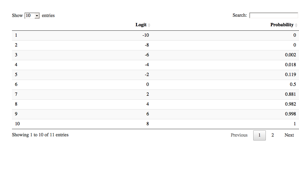
Conversion table
Here’s a look up table for the conversion:
logit_seq <- seq(-10, 10, by = 2)
prob_seq <- round(logit2prob(logit_seq), 3)

df <- data.frame(Logit = logit_seq,
                 Probability = prob_seq)
library(htmlTable)
htmlTable(df)
| Logit | Probability | |
|---|---|---|
| 1 | -10 | 0 |
| 2 | -8 | 0 |
| 3 | -6 | 0.002 |
| 4 | -4 | 0.018 |
| 5 | -2 | 0.119 |
| 6 | 0 | 0.5 |
| 7 | 2 | 0.881 |
| 8 | 4 | 0.982 |
| 9 | 6 | 0.998 |
| 10 | 8 | 1 |
| 11 | 10 | 1 |
A handy function is datatable, does not work in this environment however it appears.
library(DT)
datatable(df)
The package mfx provides a convenient functions to get odds out of a logistic regression (Thanks for Henry Cann’s comment for pointing that out!).
Conversion plot
More convenient for an overview is a plot like this.
library(ggplot2)


logit_seq <- seq(-10, 10, by = .1)

prob_seq <- logit2prob(logit_seq)

rm(df)

df <- data.frame(Logit = logit_seq,
                 Probability = prob_seq)

ggplot(df) +
  aes(x = logit_seq, y = prob_seq) +
  geom_point(size = 2, alpha = .3) +
  labs(x = "logit", y = "probability of success")

Takeway
The relationship between logit and probability is not linear, but of s-curve type.
The coefficients in logit form can be be treated as in normal regression in terms of computing the y-value.
Transform the logit of your y-value to probability to get a sense of the probability of the modeled event.
Happy glming!
sessionInfo
sessionInfo()
## R version 3.3.2 (2016-10-31)
## Platform: x86_64-apple-darwin13.4.0 (64-bit)
## Running under: macOS Sierra 10.12.4
##
## locale:
## [1] en_US.UTF-8/en_US.UTF-8/en_US.UTF-8/C/en_US.UTF-8/en_US.UTF-8
##
## attached base packages:
## [1] stats     graphics  grDevices utils     datasets  methods   base
##
## other attached packages:
## [1] ggplot2_2.2.1 DT_0.2        htmlTable_1.9
##
## loaded via a namespace (and not attached):
##  [1] Rcpp_0.12.10        knitr_1.16          magrittr_1.5
##  [4] munsell_0.4.3       colorspace_1.3-2    R6_2.2.1
##  [7] rlang_0.1           plyr_1.8.4          stringr_1.2.0
## [10] highr_0.6           dplyr_0.5.0         tools_3.3.2
## [13] grid_3.3.2          webshot_0.4.0       gtable_0.2.0
## [16] checkmate_1.8.2     DBI_0.6-1           htmltools_0.3.6
## [19] yaml_2.1.14         lazyeval_0.2.0.9000 assertthat_0.2.0
## [22] rprojroot_1.2       digest_0.6.12       tibble_1.3.0.9002
## [25] htmlwidgets_0.8     rsconnect_0.8       evaluate_0.10
## [28] rmarkdown_1.5       labeling_0.3        stringi_1.1.5
## [31] scales_0.4.1        backports_1.0.5     jsonlite_1.4