reading time: 5-10 min.
Cohen’s d is a widely known and extensively used measure of effect size. That is, d is used to gauge how strong an effect is (given the fact that the effect exists). For example, one way to estimate d is as follows:
data(tips, package = "reshape2")
library(compute.es)
t1 <- t.test(tip ~ sex, data = tips)
t1$statistic
##         t
## -1.489536
table(tips$sex)
##
## Female   Male
##     87    157
tes(t1$statistic, 87, 157)
## Mean Differences ES:
##
##  d [ 95 %CI] = -0.2 [ -0.46 , 0.06 ]
##   var(d) = 0.02
##   p-value(d) = 0.14
##   U3(d) = 42.11 %
##   CLES(d) = 44.4 %
##   Cliff's Delta = -0.11
##
##  g [ 95 %CI] = -0.2 [ -0.46 , 0.06 ]
##   var(g) = 0.02
##   p-value(g) = 0.14
##   U3(g) = 42.13 %
##   CLES(g) = 44.42 %
##
##  Correlation ES:
##
##  r [ 95 %CI] = 0.1 [ -0.03 , 0.22 ]
##   var(r) = 0
##   p-value(r) = 0.14
##
##  z [ 95 %CI] = 0.1 [ -0.03 , 0.22 ]
##   var(z) = 0
##   p-value(z) = 0.14
##
##  Odds Ratio ES:
##
##  OR [ 95 %CI] = 0.7 [ 0.43 , 1.12 ]
##   p-value(OR) = 0.14
##
##  Log OR [ 95 %CI] = -0.36 [ -0.84 , 0.12 ]
##   var(lOR) = 0.06
##   p-value(Log OR) = 0.14
##
##  Other:
##
##  NNT = -19.61
##  Total N = 244
However, what does Cohen’s d mean eventually?
Ok, the formula of d is well-known. In essence, d is computed as the difference between two means, normalized by the average variation. So one could say: “Wow, the experimental group was about 0.5 sd above the control! Jippaa!”” Not sure whether “lay persons”” would follow.
How can one get a more intuitive understanding of d?
A first step is to recognize that the two distributions overlap less if d gets larger.
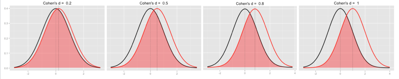
As a sidenote: The size of the overlap can be computed quite easily:
- Take the half of the mean difference (eg., 1-0 = 1, divided by 2 equals 0.5)
- This is exactly the point where the two curves intersect (see figure)
- Assuming that the “left”” mean is zero, you will now have a quantile at 0.5
- Look up the percentile of that quantile (or in R, use pnorm()), ie., about 0.70
- Now you know that at the right of this point, there is about 0.30 of probability mass
So in total, the overlap area amounts to 0.60 ie. 60%. Ok, good, but what does overlap really means?
A more approachable statistics is CLES. CLES stands for common language effect size. Basically, it answers the question:
“If I draw 100 guys from distribution 1 and 100 from distribution 2, what is the chance that guy from 1 has a higher value than guy from 2?”
Ah! This makes sense! At least to me. We have now an observable, practical description of what this effect size means.
From our example above: The chance is 44% that a woman will tip more willingly than a man. To put it differently: Pick 100 pairs (woman/man). On average, 44 of these women will tip more than their male counterpart.