A chloropleth map is a geographic map where statistical information are mapped to certain areas. Let’s plot such a chloropleth map in this post.
Packages
library(sf)
library(stringr)
library(tidyverse)
library(readxl)
Geo data
Best place to get German geo data is from the “Bundesamt für Kartografie und Geodäsie (BKG)”. One may basically use the data for a purposes unless it is against the law. I have downloaded the data 2017-10-09. More specifically, we are looking at the “Verwaltungsgebiete” (vg), that is, the administrative areas of the country, ie., counties, states etc.
Look for the “Verwaltungsgebiete”. On this page you’ll get the geo data scaled 1:2,500,000. This material includes area map of the whole state (hence sta, see below) of Germany.
It’s quite a bit of data. Download it, unzip it and adapt your path variables accordingly. The data is stores as shape files, a standard format for open geo data.
my_path_vg2500_sta <- "~/Documents/datasets/geo_maps/vg2500/vg2500_sta.shp"
file.exists(my_path_vg2500_sta)
#> [1] TRUE
vg2500_sta <- st_read(my_path_vg2500_sta)
#> Reading layer `vg2500_sta' from data source `/Users/sebastiansauer/Documents/datasets/geo_maps/vg2500/vg2500_sta.shp' using driver `ESRI Shapefile'
#> Simple feature collection with 3 features and 4 fields
#> geometry type:  MULTIPOLYGON
#> dimension:      XY
#> bbox:           xmin: 280353.1 ymin: 5235878 xmax: 921021.2 ymax: 6104656
#> epsg (SRID):    NA
#> proj4string:    +proj=utm +zone=32 +ellps=GRS80 +units=m +no_defs
vg2500_sta %>%
  slice(2:3) %>%  # line 1 are coastal "water" areas
  ggplot() +
  geom_sf()
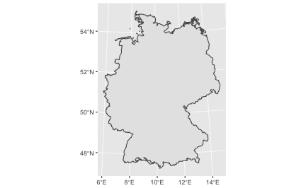
That was easy, right? The sf package fits nicely with the tidyverse. Hence not much to learn in that regard. I am not saying that geo data is simple, quite the contrary. But luckily the R functions fit in a well known schema.
For instance, let’s remove the axis labels and let’s fill the country with some different color. Hm, what’s the color of Germany? Grey? Black (color of the leading party)? Black-red-gold?
vg2500_sta %>%
  slice(2:3) %>%
  ggplot() +
  geom_sf(fill = "grey40") +
  theme_void()
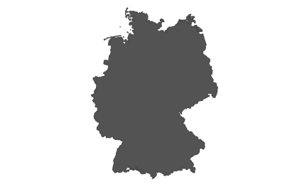
Now, let’s have a look to the more hi-res data. There a a number of files. We will first use the files with borders, or, geometrically, lines:
my_path_vg250_L <- "~/Documents/datasets/geo_maps/vg250/vg250_kompakt/VG250_L.shp"  # de for Germany (country code), and L as in lines
vg_250_L <- st_read(my_path_vg250_L)
#> Reading layer `VG250_L' from data source `/Users/sebastiansauer/Documents/datasets/geo_maps/vg250/vg250_kompakt/VG250_L.shp' using driver `ESRI Shapefile'
#> Simple feature collection with 36292 features and 3 fields
#> geometry type:  LINESTRING
#> dimension:      XY
#> bbox:           xmin: 280371.1 ymin: 5235856 xmax: 921292.4 ymax: 6106244
#> epsg (SRID):    NA
#> proj4string:    +proj=utm +zone=32 +ellps=GRS80 +units=m +no_defs
head(vg_250_L)
#> Simple feature collection with 6 features and 3 fields
#> geometry type:  LINESTRING
#> dimension:      XY
#> bbox:           xmin: 312391.4 ymin: 5271478 xmax: 897074.9 ymax: 5657429
#> epsg (SRID):    NA
#> proj4string:    +proj=utm +zone=32 +ellps=GRS80 +units=m +no_defs
#>   AGZ RDG GM5                       geometry
#> 1   1   1   0 LINESTRING (439205.44865438...
#> 2   1   1   0 LINESTRING (316806.88365514...
#> 3   1   1   0 LINESTRING (390438.74675088...
#> 4   1   1   0 LINESTRING (392662.34014679...
#> 5   1   1   0 LINESTRING (826537.76462522...
#> 6   1   1   0 LINESTRING (896720.92151288...
st_read comes as a friend, smooth and hasslefree. All geo data is stored in one column: geometry. The other columns provide district data. The most important one here for us at this point is AGZ meaning type of border. Value 1 is national border. All right then, let’s draw the country borders.
vg_250_L %>%
  filter(AGZ == 1) %>%
  ggplot +
  geom_sf()
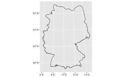
Note that this time, we have lines, no areas, hence we cannot fill the country with some color.
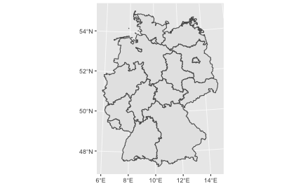
Now, let’s look at the larger Verwaltungsgebiete of Germany, they are:
- Land (state;
lan) - Regierungsbezirk (legislative area,
rbz) - Kreis (county,
krs)
Same principle as before:
my_path_vg2500_lan <- "~/Documents/datasets/geo_maps/vg2500/vg2500_lan.shp"
file.exists(my_path_vg2500_sta)
#> [1] TRUE
vg2500_lan <- st_read(my_path_vg2500_lan)
#> Reading layer `vg2500_lan' from data source `/Users/sebastiansauer/Documents/datasets/geo_maps/vg2500/vg2500_lan.shp' using driver `ESRI Shapefile'
#> Simple feature collection with 16 features and 4 fields
#> geometry type:  MULTIPOLYGON
#> dimension:      XY
#> bbox:           xmin: 280353.1 ymin: 5235878 xmax: 921021.2 ymax: 6101335
#> epsg (SRID):    NA
#> proj4string:    +proj=utm +zone=32 +ellps=GRS80 +units=m +no_defs
head(vg2500_lan)
#> Simple feature collection with 6 features and 4 fields
#> geometry type:  MULTIPOLYGON
#> dimension:      XY
#> bbox:           xmin: 280353.1 ymin: 5423990 xmax: 674168.3 ymax: 5979709
#> epsg (SRID):    NA
#> proj4string:    +proj=utm +zone=32 +ellps=GRS80 +units=m +no_defs
#>   ADE RS         RS_0                 GEN                       geometry
#> 1   2 02 020000000000             Hamburg MULTIPOLYGON (((578594.2157...
#> 2   2 03 030000000000       Niedersachsen MULTIPOLYGON (((354762.3478...
#> 3   2 04 040000000000              Bremen MULTIPOLYGON (((468599.9059...
#> 4   2 05 050000000000 Nordrhein-Westfalen MULTIPOLYGON (((477387.5570...
#> 5   2 06 060000000000              Hessen MULTIPOLYGON (((546606.7604...
#> 6   2 07 070000000000     Rheinland-Pfalz MULTIPOLYGON (((418854.5347...
vg2500_lan %>%
  ggplot() +
  geom_sf()
my_path_vg2500_rbz <- "~/Documents/datasets/geo_maps/vg2500/vg2500_rbz.shp"
file.exists(my_path_vg2500_sta)
#> [1] TRUE
vg2500_rbz <- st_read(my_path_vg2500_rbz)
#> Reading layer `vg2500_rbz' from data source `/Users/sebastiansauer/Documents/datasets/geo_maps/vg2500/vg2500_rbz.shp' using driver `ESRI Shapefile'
#> Simple feature collection with 19 features and 4 fields
#> geometry type:  MULTIPOLYGON
#> dimension:      XY
#> bbox:           xmin: 280353.1 ymin: 5235878 xmax: 855553.1 ymax: 5820162
#> epsg (SRID):    NA
#> proj4string:    +proj=utm +zone=32 +ellps=GRS80 +units=m +no_defs
head(vg2500_rbz)
#> Simple feature collection with 6 features and 4 fields
#> geometry type:  MULTIPOLYGON
#> dimension:      XY
#> bbox:           xmin: 280353.1 ymin: 5471359 xmax: 553250.7 ymax: 5820162
#> epsg (SRID):    NA
#> proj4string:    +proj=utm +zone=32 +ellps=GRS80 +units=m +no_defs
#>   ADE  RS         RS_0        GEN                       geometry
#> 1   3 051 051000000000 Düsseldorf MULTIPOLYGON (((308582.1649...
#> 2   3 053 053000000000       Köln MULTIPOLYGON (((384170.0176...
#> 3   3 055 055000000000    Münster MULTIPOLYGON (((415321.4839...
#> 4   3 057 057000000000    Detmold MULTIPOLYGON (((477387.5570...
#> 5   3 059 059000000000   Arnsberg MULTIPOLYGON (((397616.4384...
#> 6   3 064 064000000000  Darmstadt MULTIPOLYGON (((506866.1477...
vg2500_rbz %>%
  ggplot() +
  geom_sf()
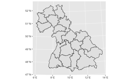
Hmm, this one looks weird; some areas appear to be lost in action.
vg2500_rbz %>% pull(GEN)
#>  [1] Düsseldorf    Köln          Münster       Detmold       Arnsberg
#>  [6] Darmstadt     Gießen        Kassel        Stuttgart     Karlsruhe
#> [11] Freiburg      Tübingen      Oberbayern    Niederbayern  Oberpfalz
#> [16] Oberfranken   Mittelfranken Unterfranken  Schwaben
#> 19 Levels: Arnsberg Darmstadt Detmold Düsseldorf Freiburg ... Unterfranken
Only 19 Kreises are reported, and no values from northern or eastern part of the country. Strange.
my_path_vg2500_krs <- "~/Documents/datasets/geo_maps/vg2500/vg2500_krs.shp"
file.exists(my_path_vg2500_krs)
#> [1] TRUE
vg2500_krs <- st_read(my_path_vg2500_krs)
#> Reading layer `vg2500_krs' from data source `/Users/sebastiansauer/Documents/datasets/geo_maps/vg2500/vg2500_krs.shp' using driver `ESRI Shapefile'
#> Simple feature collection with 401 features and 4 fields
#> geometry type:  MULTIPOLYGON
#> dimension:      XY
#> bbox:           xmin: 280353.1 ymin: 5235878 xmax: 921021.2 ymax: 6101335
#> epsg (SRID):    NA
#> proj4string:    +proj=utm +zone=32 +ellps=GRS80 +units=m +no_defs
head(vg2500_krs)
#> Simple feature collection with 6 features and 4 fields
#> geometry type:  MULTIPOLYGON
#> dimension:      XY
#> bbox:           xmin: 478836.8 ymin: 5913378 xmax: 629246.8 ymax: 6075267
#> epsg (SRID):    NA
#> proj4string:    +proj=utm +zone=32 +ellps=GRS80 +units=m +no_defs
#>   ADE    RS         RS_0                 GEN
#> 1   4 01001 010010000000           Flensburg
#> 2   4 01002 010020000000                Kiel
#> 3   4 01003 010030000000              Lübeck
#> 4   4 01004 010040000000          Neumünster
#> 5   4 01051 010510000000        Dithmarschen
#> 6   4 01053 010530000000 Herzogtum Lauenburg
#>                         geometry
#> 1 MULTIPOLYGON (((531470.9568...
#> 2 MULTIPOLYGON (((577310.2796...
#> 3 MULTIPOLYGON (((624204.4378...
#> 4 MULTIPOLYGON (((567602.4930...
#> 5 MULTIPOLYGON (((479551.7420...
#> 6 MULTIPOLYGON (((616195.6437...
vg2500_krs %>%
  ggplot() +
  geom_sf()
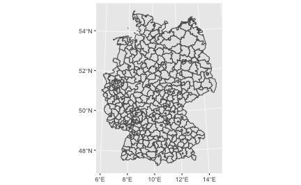
Ok, that’s complete. How many of those “Kreise” do we have? Well, 401, that’s the number of rows we have in the data frame.
unemployment rates
These data can as well be fetched from official sites, that’s in this case the “Bundesämter für Statistik”. We consider here the unemployment rates of German counties for 2016 as provided by this agency.
unemp_file <- "~/Documents/datasets/Strukturdaten_de/GUEST_9559782118415_Arbeitslosenquote_2016.csv"
file.exists(unemp_file)
#> [1] TRUE

unemp_de_raw <- read_csv2(unemp_file)
unemp_de_raw %>%
  mutate(Wert = as.numeric(Wert)) %>%
  separate(Name, into = c("Name", "vg_type"), sep = ",") -> unemp_de

unemp_de %>%
  filter(Name == "Nürnberg")
#> # A tibble: 1 x 4
#>   Schluessel     Name vg_type  Wert
#>        <chr>    <chr>   <chr> <dbl>
#> 1      09564 Nürnberg    <NA>   6.6
Match unemployment to geo data
Presumingly, we will not have a perfect match, but let’s see how good or bad it will be out of the box.
vg2500_krs %>%
  mutate(GEN = as.character(GEN)) %>%
  left_join(unemp_de, by = c("GEN" = "Name")) -> vg2500_krs_unemp
Let’s plot the unemployment rates per administrative area.
vg2500_krs_unemp %>%
  ggplot() +
  geom_sf(aes(fill = Wert)) +
  labs(fill = "unemployment\nrate") +
  scale_fill_distiller(palette = "RdYlGn") +
  theme_void()
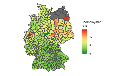
Appeared to work pretty well; but I have not checked the details yet. For the top right state, Mecklenburg-Vorpommern, no data were made available by the agency.