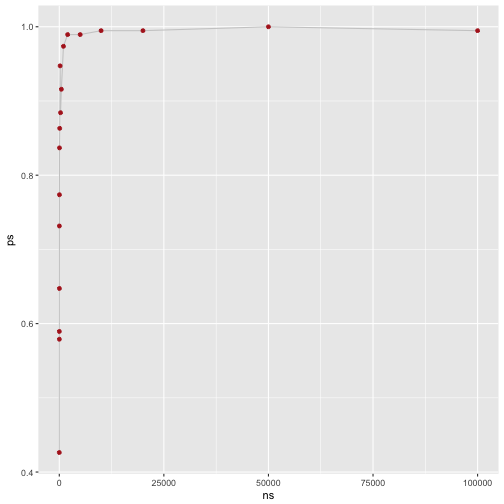
It is well-known that the notorious p-values is sensitive to sample size: The larger the sample, the more bound the p-value is to fall below the magic number of .05.

Of course, the p-value is also a function of the effect size, eg., the distance between two means and the respective variances. But still, the p-values tends to become significant in the face of larges samples, and non-significant otherwise.

Theoretically, quite simple and well understood. But let’s take the test of “real” data and do a simulation to demonstrate or test this behavior.

First, load some required packages

library(tidyverse)

Simulate data with large sample size

Next, we simulate data: A data frame of 20 cols and many rows (1e06, ie., 1 million). We should also make sure that the null hypothesis is false in our data. To that end, we let the mean values of the columns vary somewhat.

k <- 20
n <- 1e06
df <- data.frame(replicate(k,rnorm(n = n, mean = rnorm(1, 0, 1), sd = 1)))

Now let’s compute t-tests for each and every combination (cartesian product of all combinations). We will save the resulting p-values in a (square) matrix.

m <- matrix(nrow = k, ncol = k)


for (i in seq_len(ncol(df))) {
  for (j in seq_len(ncol(df))) {
    m[i, j] <- t.test(df[i], df[j])$p.value
  }
}

One half of the matrix is redundant, as the matrix is symmetric. The same reasoning applies for the diagonal. Let’s take out the redundant elements.

m[lower.tri(m)] <- NA
m[diag(m)] <- NA

Let’s come up with a logical matrix indicating whether one cell (ie., one t-test) indicates a significant t-test (TRUE) or not (FALSE).

m_significant <- apply(m, c(1,2), function(x) x < .05)

Finally, let’s count the number of significant results, and sum then up.

m_significant %>% sum(TRUE, na.rm = TRUE)

## [1] 191

The number of different tests is \((k*k - k)/2\).

Which amounts, in this case to

(k*k-20)/2

## [1] 190

Hence, all tests are significant.

rm(df)

Simulate data with small sample size

Now, we repeat the same thing with a small sample.

simulate_ps <- function(n = 1e06, k = 20){
  
  # arguments:
  # n: number of rows
  # k: number of columns
  # returns: proportion of significant (p<.05) t-tests

set.seed(42)  
  
# simulate data
df <- data.frame(replicate(k,rnorm(n = n, mean = rnorm(1, 0, 1), sd = 1)))

# matrix for t-test results
m <- matrix(nrow = k, ncol = k)

# cartesian product of all t-tests
for (i in seq_len(ncol(df))) {
  for (j in seq_len(ncol(df))) {
    m[i, j] <- t.test(df[i], df[j])$p.value
  }
}

# take-out redundant cells
m[lower.tri(m)] <- NA
m[diag(m)] <- NA

# compute matrix to count number of significant t-tests
m_significant <- apply(m, c(1,2), function(x) x < .05)


# count
sum_significant <- m_significant %>% sum(TRUE, na.rm = TRUE)

sum_distinct_tests <- (k*k - k)/2

prop_significant <- sum_significant / sum_distinct_tests

rm(df)
return(prop_significant)

}

simulate_ps(n = 10, k = 20)

## [1] 0.5894737

Play around

Now, we can play around a bit.

ns <- c(5, 10, 15, 20, 30, 40, 50, 100, 200, 300, 500, 1000, 2000, 5000, 10000, 2e04, 5e04, 1e05)

ps <- vector(mode = "numeric", length = length(ns))

for (i in seq_along(ns)){
  ps[i] <- simulate_ps(n = ns[i], k = 20)
  print(ps[i])
}

## [1] 0.4263158
## [1] 0.5894737
## [1] 0.5789474
## [1] 0.7315789
## [1] 0.6473684
## [1] 0.7736842
## [1] 0.8368421
## [1] 0.8631579
## [1] 0.9473684
## [1] 0.8842105
## [1] 0.9157895
## [1] 0.9736842
## [1] 0.9894737
## [1] 0.9894737
## [1] 0.9947368
## [1] 0.9947368
## [1] 1
## [1] 0.9947368

Finally, let’s plot that:

data_frame(
  ns = ns,
  ps = ps
)  %>% 
  ggplot +
  aes(x = ns, y = ps) +
  geom_line(color = "gray80") +
  geom_point(color = "firebrick")

Thus, our result appears reasonable: The larger the sample size (ns), the higher the proportion of ps (ps).