Let’s draw a map of Bavaria, a state of Germany, in this post.
Packages
library(tidyverse)
library(maptools)
library(sf)
library(RColorBrewer)
library(ggmap)
library(viridis)
library(stringr)
Data
Let’s get the data first. Basically, we need to data files:
- the shape file, ie., a geographic details of state borders and points of interest
- the semantic information to points of interest eg., town names
Shape file
The shape file can be downloaded from this source: http://www.metaspatial.net/download/plz.tar.gz
This site also looks great to get geospatial data.
These data are PD as stated here. Download and unpack the data. Let’s assume that the data are stored in a path called my_path. See for instance in my case:
# replace the following path with your path:
my_path <- "/Users/sebastiansauer/Documents/Datensaetze/plz/"
my_shape <- "post_pl.shp"

shape_dest <- paste0(my_path, my_shape)
file.exists(shape_dest)
#> [1] TRUE
Parse the shape data:
de_shape <- sf::st_read(shape_dest)  # "de" is for Germany
#> Reading layer `post_pl' from data source `/Users/sebastiansauer/Documents/Datensaetze/plz/post_pl.shp' using driver `ESRI Shapefile'
#> Simple feature collection with 8270 features and 3 fields
#> geometry type:  MULTIPOLYGON
#> dimension:      XY
#> bbox:           xmin: 5.866286 ymin: 47.2736 xmax: 15.04863 ymax: 55.05826
#> epsg (SRID):    NA
#> proj4string:    NA
Check the result:
head(de_shape)
#> Simple feature collection with 6 features and 3 fields
#> geometry type:  MULTIPOLYGON
#> dimension:      XY
#> bbox:           xmin: 13.69598 ymin: 51.02433 xmax: 13.91312 ymax: 51.14665
#> epsg (SRID):    NA
#> proj4string:    NA
#>   PLZ99 PLZ99_N PLZORT99                       geometry
#> 1 01067    1067  Dresden MULTIPOLYGON (((13.7189358 ...
#> 2 01069    1069  Dresden MULTIPOLYGON (((13.74983892...
#> 3 01097    1097  Dresden MULTIPOLYGON (((13.727583 5...
#> 4 01099    1099  Dresden MULTIPOLYGON (((13.82015592...
#> 5 01109    1109  Dresden MULTIPOLYGON (((13.75953588...
#> 6 01127    1127  Dresden MULTIPOLYGON (((13.72007952...
de_shape$PLZORT99 %>% head
#> [1] Dresden Dresden Dresden Dresden Dresden Dresden
#> 6359 Levels: Aach Aachen Aalen Aarbergen Abenberg Abensberg ... \xdfxheim
Note that the file contains semantic data, too (zip code, town names).
Some encoding problems. More often than not, text data is in the wrong format. Blind guessing: Data was stored on a Windows machine, hence in Latin1. My system assumes UTF-8, so culture clash is to expected. Let’s try to fix.
de_shape$PLZORT99 <- as.character(de_shape$PLZORT99)
Encoding(de_shape$PLZORT99) <- "latin1"
slice(de_shape$PLZORT99, 90:100)
#> Error in UseMethod("slice_"): no applicable method for 'slice_' applied to an object of class "character"
Ok, fixed.
Shape semantics
“Shape semantics” is a rather fancy word for the county/community/town names. We can access the data here.
Download and unzip the data, then move it to my_path. The German word for “zip code” is “PLZ”, so that’s why I call it my_plz:
my_plz <- "PLZ_Ort_Long_Lat_Land_DE.txt"
de_plz <- paste0(my_path, my_plz)
file.exists(de_plz)
#> [1] TRUE

plz_df <- read_tsv(file = de_plz, col_names = FALSE)  # tab separated data
In the help file from the downloaded data, we find some explanation as to the columns:
plz_df <- plz_df %>%
  rename(country_code = X1,
         postal_code = X2,
         place_name = X3,
         state = X4,
         state_code = X5,
         county = X6,
         county_code = X7,
         community = X8,
         community_code = X9,
         lat = X10,
         long = X11,
         accuracy = X12)  # accuracy of lat/lng from 1=estimated to 6=centroid


glimpse(plz_df)
#> Observations: 16,481
#> Variables: 12
#> $ country_code   <chr> "DE", "DE", "DE", "DE", "DE", "DE", "DE", "DE",...
#> $ postal_code    <chr> "01945", "01945", "01945", "01945", "01945", "0...
#> $ place_name     <chr> "Hohenbocka", "Lindenau", "Schwarzbach", "Grüne...
#> $ state          <chr> "Brandenburg", "Brandenburg", "Brandenburg", "B...
#> $ state_code     <chr> "BB", "BB", "BB", "BB", "BB", "BB", "BB", "BB",...
#> $ county         <chr> NA, NA, NA, NA, NA, NA, NA, NA, NA, NA, NA, NA,...
#> $ county_code    <chr> "00", "00", "00", "00", "00", "00", "00", "00",...
#> $ community      <chr> "Landkreis Oberspreewald-Lausitz", "Landkreis O...
#> $ community_code <int> 12066, 12066, 12066, 12066, 12066, 12066, 12066...
#> $ lat            <dbl> 51.4, 51.4, 51.5, 51.4, 51.4, 51.5, 51.4, 51.4,...
#> $ long           <dbl> 14.0, 13.7, 13.9, 14.0, 13.9, 13.9, 13.9, 13.7,...
#> $ accuracy       <chr> NA, NA, NA, NA, NA, NA, NA, NA, NA, NA, NA, NA,...
Test it
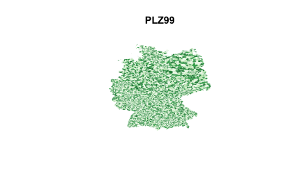
Now, enough of grey theory! Unfortunately, I don’t know any nice Hamlet citation here, which would certainly be impressive.
my_col <- sample(1:7, length(de_shape), replace = T)
plot(de_shape[c("PLZ99", "geometry")],
     col = brewer.pal(7, "Greens")[my_col], border = F)
Filter Bavaria
plz_bavaria <- plz_df %>%
  filter(state == "Bayern")

plz_bavaria_vec <- plz_bavaria$postal_code
Easy; ~2259 zip codes in Bavaria.
Now let’s filter the shape file.
my_rows <- de_shape$PLZ99 %in% plz_bavaria_vec
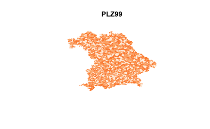
And plot Bavaria:
my_col <- sample(1:7, length(de_shape), replace = T)

bav_data <- de_shape[my_rows,c("PLZ99", "geometry")]
plot(bav_data,
     col = brewer.pal(7, "Oranges")[my_col], border = F)
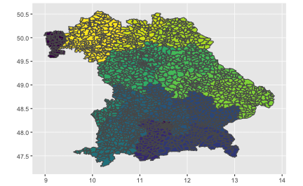
Now plot with ggplot2
bav_data$PLZ2 <- str_extract(bav_data$PLZ99, "\\d\\d")


ggplot(data = bav_data) +
  geom_sf(aes(fill = PLZ2)) +
  scale_fill_viridis_d() +
  guides(fill = FALSE) -> p_bavaria
p_bavaria
Sample some counties
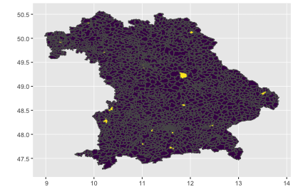
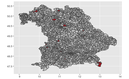
FWIW, let’s sample some counties, and fill them in a distinct color.
bav_data$PLZ_sample <- sample(c(0,1),
                              size = nrow(bav_data),
                              prob = c(.99, .01),
                              replace = TRUE)


ggplot(data = bav_data) +
  geom_sf(aes(fill = PLZ_sample)) +
  scale_fill_viridis() +
  guides(fill = FALSE) -> p_bavaria2
p_bavaria2
Let’s define our own palette:
bav_data$PLZ_sample <- sample(c(0,1),
                              size = nrow(bav_data),
                              prob = c(.99, .01),
                              replace = TRUE) %>% factor
my_pal <- c("grey80", "firebrick")
ggplot(data = bav_data) +
  geom_sf(aes(fill = PLZ_sample)) +
  scale_fill_manual(values = my_pal) +
  guides(fill = FALSE) -> p_bavaria3
p_bavaria3
Bigger visual chunks
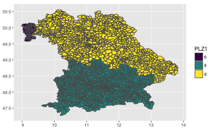
Let’s cut the polygons in bigger chunks, say, according to the first digit in the zip code.
bav_data$PLZ1 <- str_extract(bav_data$PLZ99, "\\d")

my_pal <- c("grey80", "firebrick")
ggplot(data = bav_data) +
  geom_sf(aes(fill = PLZ1)) +
  scale_fill_viridis_d() -> p_bavaria4
p_bavaria4
Happy map painting!