library(tidyverse)stipro-beschreiben
Question
Beschreiben Sie den Datensatz mtcars!
Nehmen Sie Bezug auf die Forschungsfrage “PS-Zahl hat einen Einfluss auf den Spritverbrauch”.
Solution
library(datawizard)
tab1 <- describe_distribution(mtcars)
tab1| Variable | Mean | SD | IQR | Min | Max | Skewness | Kurtosis | n | n_Missing |
|---|---|---|---|---|---|---|---|---|---|
| mpg | 20.090625 | 6.0269481 | 7.52500 | 10.400 | 33.900 | 0.6723771 | -0.0220063 | 32 | 0 |
| cyl | 6.187500 | 1.7859216 | 4.00000 | 4.000 | 8.000 | -0.1922609 | -1.7627939 | 32 | 0 |
| disp | 230.721875 | 123.9386938 | 221.52500 | 71.100 | 472.000 | 0.4202331 | -1.0675234 | 32 | 0 |
| hp | 146.687500 | 68.5628685 | 84.50000 | 52.000 | 335.000 | 0.7994067 | 0.2752116 | 32 | 0 |
| drat | 3.596563 | 0.5346787 | 0.84000 | 2.760 | 4.930 | 0.2927802 | -0.4504325 | 32 | 0 |
| wt | 3.217250 | 0.9784574 | 1.18625 | 1.513 | 5.424 | 0.4659161 | 0.4165947 | 32 | 0 |
| qsec | 17.848750 | 1.7869432 | 2.02250 | 14.500 | 22.900 | 0.4063466 | 0.8649307 | 32 | 0 |
| vs | 0.437500 | 0.5040161 | 1.00000 | 0.000 | 1.000 | 0.2645418 | -2.0632731 | 32 | 0 |
| am | 0.406250 | 0.4989909 | 1.00000 | 0.000 | 1.000 | 0.4008089 | -1.9665503 | 32 | 0 |
| gear | 3.687500 | 0.7378041 | 1.00000 | 3.000 | 5.000 | 0.5823086 | -0.8952916 | 32 | 0 |
| carb | 2.812500 | 1.6152000 | 2.00000 | 1.000 | 8.000 | 1.1570911 | 2.0200593 | 32 | 0 |
Wenn Sie es in Word exportieren wollen:
library(flextable)
flextable(tab1)
Variable | Mean | SD | IQR | Min | Max | Skewness | Kurtosis | n | n_Missing |
|---|---|---|---|---|---|---|---|---|---|
mpg | 20.090625 | 6.0269481 | 7.52500 | 10.400 | 33.900 | 0.6723771 | -0.02200629 | 32 | 0 |
cyl | 6.187500 | 1.7859216 | 4.00000 | 4.000 | 8.000 | -0.1922609 | -1.76279390 | 32 | 0 |
disp | 230.721875 | 123.9386938 | 221.52500 | 71.100 | 472.000 | 0.4202331 | -1.06752340 | 32 | 0 |
hp | 146.687500 | 68.5628685 | 84.50000 | 52.000 | 335.000 | 0.7994067 | 0.27521159 | 32 | 0 |
drat | 3.596563 | 0.5346787 | 0.84000 | 2.760 | 4.930 | 0.2927802 | -0.45043245 | 32 | 0 |
wt | 3.217250 | 0.9784574 | 1.18625 | 1.513 | 5.424 | 0.4659161 | 0.41659467 | 32 | 0 |
qsec | 17.848750 | 1.7869432 | 2.02250 | 14.500 | 22.900 | 0.4063466 | 0.86493065 | 32 | 0 |
vs | 0.437500 | 0.5040161 | 1.00000 | 0.000 | 1.000 | 0.2645418 | -2.06327313 | 32 | 0 |
am | 0.406250 | 0.4989909 | 1.00000 | 0.000 | 1.000 | 0.4008089 | -1.96655033 | 32 | 0 |
gear | 3.687500 | 0.7378041 | 1.00000 | 3.000 | 5.000 | 0.5823086 | -0.89529161 | 32 | 0 |
carb | 2.812500 | 1.6152000 | 2.00000 | 1.000 | 8.000 | 1.1570911 | 2.02005931 | 32 | 0 |
Aber wie wird man die nervigen Dezimalstellen los? Zwei reichen völlig.
library(janitor)

tab1 <-
  tab1 %>%
adorn_rounding(digits = 2)flextable(tab1)Variable | Mean | SD | IQR | Min | Max | Skewness | Kurtosis | n | n_Missing |
|---|---|---|---|---|---|---|---|---|---|
mpg | 20.09 | 6.03 | 7.53 | 10.40 | 33.90 | 0.67 | -0.02 | 32 | 0 |
cyl | 6.19 | 1.79 | 4.00 | 4.00 | 8.00 | -0.19 | -1.76 | 32 | 0 |
disp | 230.72 | 123.94 | 221.52 | 71.10 | 472.00 | 0.42 | -1.07 | 32 | 0 |
hp | 146.69 | 68.56 | 84.50 | 52.00 | 335.00 | 0.80 | 0.28 | 32 | 0 |
drat | 3.60 | 0.53 | 0.84 | 2.76 | 4.93 | 0.29 | -0.45 | 32 | 0 |
wt | 3.22 | 0.98 | 1.19 | 1.51 | 5.42 | 0.47 | 0.42 | 32 | 0 |
qsec | 17.85 | 1.79 | 2.02 | 14.50 | 22.90 | 0.41 | 0.86 | 32 | 0 |
vs | 0.44 | 0.50 | 1.00 | 0.00 | 1.00 | 0.26 | -2.06 | 32 | 0 |
am | 0.41 | 0.50 | 1.00 | 0.00 | 1.00 | 0.40 | -1.97 | 32 | 0 |
gear | 3.69 | 0.74 | 1.00 | 3.00 | 5.00 | 0.58 | -0.90 | 32 | 0 |
carb | 2.81 | 1.62 | 2.00 | 1.00 | 8.00 | 1.16 | 2.02 | 32 | 0 |
S. hier zum Export in eine Word-Tabelle.
Könnte also so aussehen:
save_as_docx(tab1, path = "tab1.docx")Die Verteilung der AV:
ggplot(mtcars) +
  aes(x = mpg) +
  geom_histogram()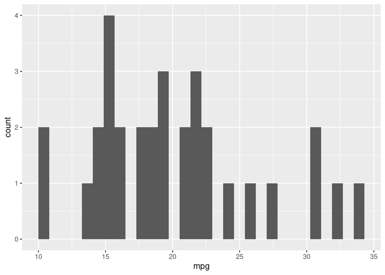
Aufgabenname: stipro-beschreiben
Meta-information
extype: string exsolution: NA exname: stipro-beschreiben expoints: 1