---
exname: geom-point1
extype: schoice
exsolution: 64
exshuffle: no
categories:
- probability
- simulation
- distributions
- bayes
- qm2
- qm2-pruefung2023
date: '2022-11-05'
title: priori-streuung
---
```{r libs, include = FALSE}
library(tidyverse)
```
```{r global-knitr-options, include=FALSE}
knitr::opts_chunk$set(fig.pos = 'H',
fig.asp = 0.618,
fig.width = 4,
fig.cap = "",
fig.path = "",
echo = FALSE,
message = FALSE,
fig.show = "hold")
```
# Exercise
Welche Verteilung ist (am besten) geeignet, um Streuung ($\sigma$) zu modellieren?
Answerlist
----------
* N(0,1)
* N(1,1)
* Exp(1)
* Exp(0)
* Exp(-1)
</br>
</br>
</br>
</br>
</br>
</br>
</br>
</br>
</br>
</br>
# Solution
Answerlist
----------
* Falsch
* Falsch
* Wahr
* Falsch
* Falsch
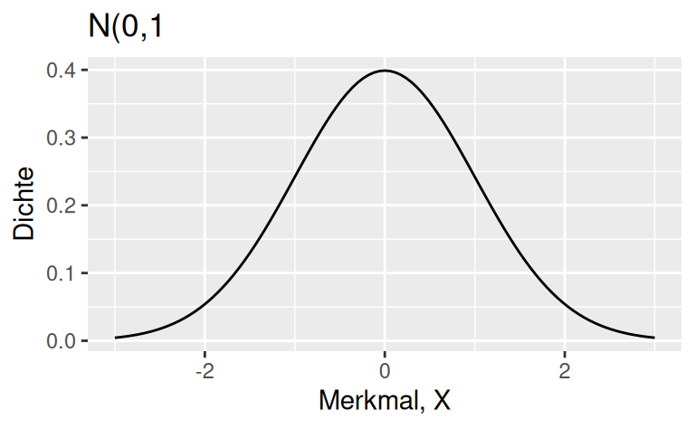
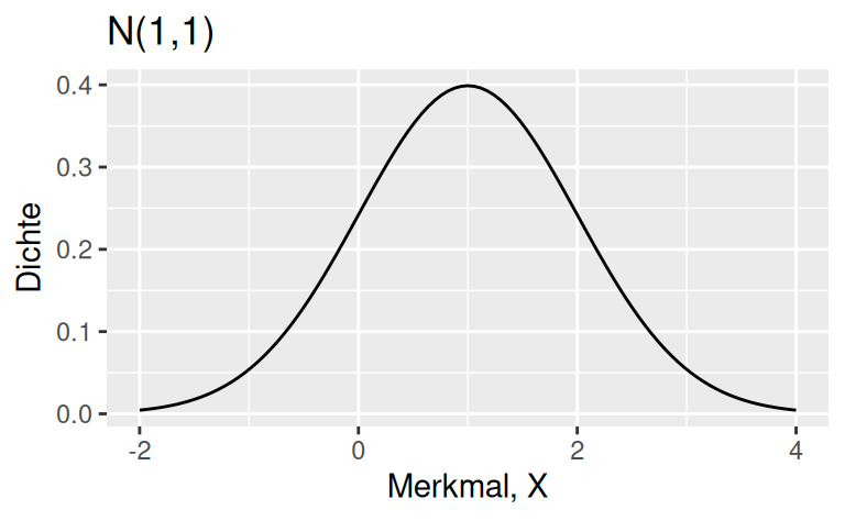
Da Streuung $\sigma$ per Definition positiv ist,
kommt eine Verteilung, die negative Werte erlaubt, nicht in Frage.
Die Normalverteilung scheidet also aus.
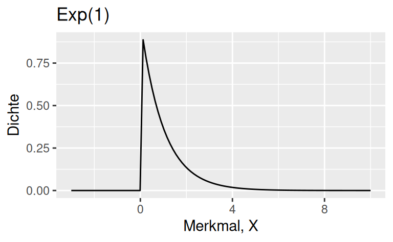
Die Rate der Exponentialverteilung regelt gleichzeitig Streuung und Mittelwert.
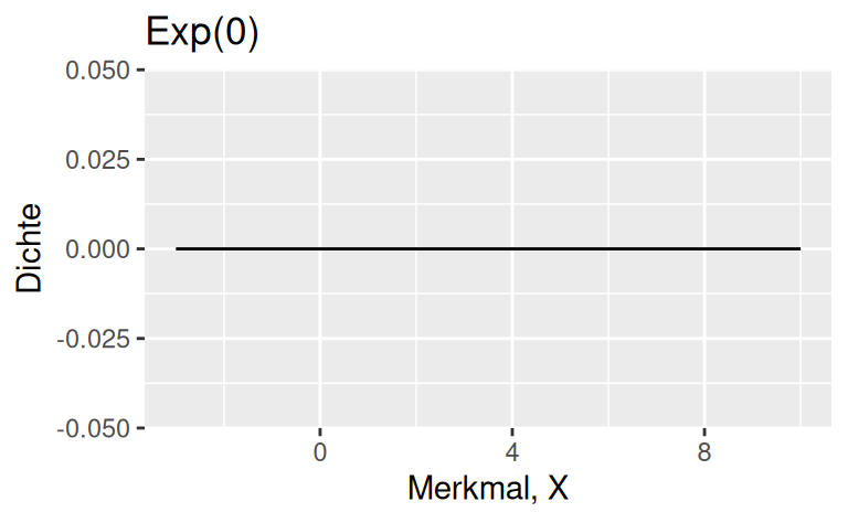
Allerdings hat $Exp(0)$ eine unendliche Streuung, was nicht wünschenswert ist.
Eine negative Rate ist für die Exponentialverteilung nicht definiert.
Normalverteilungen:
A)
</br>
$N(0,1)$:
```{r}
library(tidyverse)
ggplot(data = data.frame(x = c(-3, 3)), aes(x)) +
stat_function(fun = dnorm, n = 101) +
labs(y = "Dichte", x = "Merkmal, X",
title = "N(0,1")
```
</br>
B)
$N(1,1)$:
```{r}
ggplot(data = data.frame(x = c(-2, 4)), aes(x)) +
stat_function(fun = dnorm, n = 101, args = list(mean = 1, sd = 1)) +
labs(y = "Dichte", x = "Merkmal, X",
title = "N(1,1)")
```
Exponentialverteilungen:
C)
$Exp(1)$:
```{r}
ggplot(data = data.frame(x = c(-3, 10)), aes(x)) +
stat_function(fun = dexp, n = 101) +
labs(y = "Dichte", x = "Merkmal, X",
title = "Exp(1)")
```
D)
$Exp(0)$:
```{r}
ggplot(data = data.frame(x = c(-3, 10)), aes(x)) +
stat_function(fun = dexp, n = 101, args = list(rate = 0)) +
labs(y = "Dichte", x = "Merkmal, X",
title = "Exp(0)")
```
E)
$Exp(-1)$:
```{r}
ggplot(data = data.frame(x = c(-3, 10)), aes(x)) +
stat_function(fun = dexp, n = 101, args = list(rate = -1)) +
labs(y = "Dichte", x = "Merkmal, X",
title = "Exp(-1)")
```
---
Categories:
- probability
- simulation
- distributions
- bayes