1 Load packages
2 Wie verteilt sich das Gewicht der Autos?
3 Hängt Gewicht mit Preis zusammen?
4 Wie verteilt sich die Geschwindigkeit der Autos?
5 Hängt Preis mit Geschwindigkeit zusammen?
6 Reproducibility

1 Load packages

library(tidyverse)  # data wrangling
library(skimr)  # overview on descriptive statistics

YADCSDA in German language.

In dieser Fallstudie (YACSDA: Yet another case study of data analysis) wird der Datensatz TopGear analysiert, vor allem mit grafischen Mitteln. Es handelt sich weniger um einen “Rundumschlag” zur Beantwortung aller möglichen interessanten Fragen (oder zur Demonstration aller möglichen Analysewerkzeuge), sondern eher um einen Einblick zu einfachen explorativen Verfahren.

library(robustHD)  # Daten
data(TopGear)  # Daten aus Package laden
library(tidyverse)

1.1 Numerischer Überblick

glimpse(TopGear)
#> Rows: 297
#> Columns: 32
#> $ Maker              <fct> Alfa Romeo, Alfa Romeo, Aston Martin, Aston Martin…
#> $ Model              <fct> Giulietta, MiTo, Cygnet, DB9, DB9 Volante, V12 Zag…
#> $ Type               <fct> Giulietta 1.6 JTDM-2 105 Veloce 5d, MiTo 1.4 TB Mu…
#> $ Fuel               <fct> Diesel, Petrol, Petrol, Petrol, Petrol, Petrol, Pe…
#> $ Price              <dbl> 21250, 15155, 30995, 131995, 141995, 396000, 18999…
#> $ Cylinders          <dbl> 4, 4, 4, 12, 12, 12, 12, 8, 8, 4, 4, 4, 4, 6, 4, 6…
#> $ Displacement       <dbl> 1598, 1368, 1329, 5935, 5935, 5935, 5935, 4735, 47…
#> $ DriveWheel         <fct> Front, Front, Front, Rear, Rear, Rear, Rear, Rear,…
#> $ BHP                <dbl> 105, 105, 98, 517, 517, 510, 573, 420, 420, 86, 12…
#> $ Torque             <dbl> 236, 95, 92, 457, 457, 420, 457, 346, 346, 118, 14…
#> $ Acceleration       <dbl> 11.3, 10.7, 11.8, 4.6, 4.6, 4.2, 4.1, 4.7, 4.7, 11…
#> $ TopSpeed           <dbl> 115, 116, 106, 183, 183, 190, 183, 180, 180, 112, …
#> $ MPG                <dbl> 64, 49, 56, 19, 19, 17, 19, 20, 20, 55, 54, 61, 40…
#> $ Weight             <dbl> 1385, 1090, 988, 1785, 1890, 1680, 1739, 1630, 171…
#> $ Length             <dbl> 4351, 4063, 3078, 4720, 4720, 4385, 4720, 4385, 43…
#> $ Width              <dbl> 1798, 1720, 1680, NA, NA, 1865, 1910, 1865, 1865, …
#> $ Height             <dbl> 1465, 1446, 1500, 1282, 1282, 1250, 1294, 1260, 12…
#> $ AdaptiveHeadlights <fct> optional, optional, no, standard, standard, no, st…
#> $ AdjustableSteering <fct> standard, standard, standard, standard, standard, …
#> $ AlarmSystem        <fct> standard, standard, no/optional, no/optional, no/o…
#> $ Automatic          <fct> no, no, optional, standard, standard, no, standard…
#> $ Bluetooth          <fct> standard, standard, standard, standard, standard, …
#> $ ClimateControl     <fct> standard, optional, standard, standard, standard, …
#> $ CruiseControl      <fct> standard, standard, standard, standard, standard, …
#> $ ElectricSeats      <fct> optional, no, no, standard, standard, standard, st…
#> $ Leather            <fct> optional, optional, no, standard, standard, standa…
#> $ ParkingSensors     <fct> optional, standard, no, standard, standard, standa…
#> $ PowerSteering      <fct> standard, standard, standard, standard, standard, …
#> $ SatNav             <fct> optional, optional, standard, standard, standard, …
#> $ ESP                <fct> standard, standard, standard, standard, standard, …
#> $ Verdict            <dbl> 6, 5, 7, 7, 7, 7, 7, 8, 7, 6, 7, 6, 5, 7, 6, 7, 6,…
#> $ Origin             <fct> Europe, Europe, Europe, Europe, Europe, Europe, Eu…

TopGear %>% 
  select(Maker, Model, Type, Price, Cylinders) %>% 
  slice(1:10)

Maker	Model	Type	Price	Cylinders
Alfa Romeo	Giulietta	Giulietta 1.6 JTDM-2 105 Veloce 5d	21250	4
Alfa Romeo	MiTo	MiTo 1.4 TB MultiAir 105 Distinctive 3d	15155	4
Aston Martin	Cygnet	Cygnet 1.33 Standard 3d	30995	4
Aston Martin	DB9	DB9 6.0 517 Standard 2d 13MY	131995	12
Aston Martin	DB9 Volante	DB9 6.0 V12 517 Volante 2d 13MY	141995	12
Aston Martin	V12 Zagato	V12 Zagato 6.0 V12 Standard 2d	396000	12
Aston Martin	Vanquish	Vanquish 6.0 V12 Standard 2d	189995	12
Aston Martin	Vantage	V8 Vantage 4.7 V8 420 Standard 2d	84995	8
Aston Martin	Vantage Roadster	V8 Vantage 4.7 420 Roadster 2d	93995	8
Audi	A1	A1 1.2 TFSI 86 S line 3d	17025	4

1.2 Wie verteilen sich die Preise?

ggplot(data = TopGear,
       aes(x = Price)) +
  geom_histogram()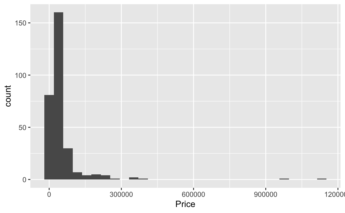

ggplot(data = TopGear,
       aes(x = log(Price))) +
  geom_histogram()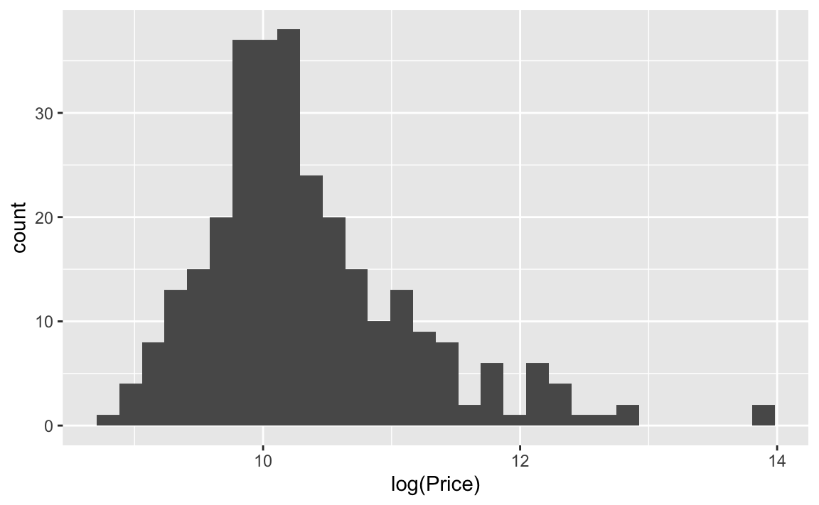

ggplot(data = TopGear,
       aes(x = log(Price))) +
  geom_density()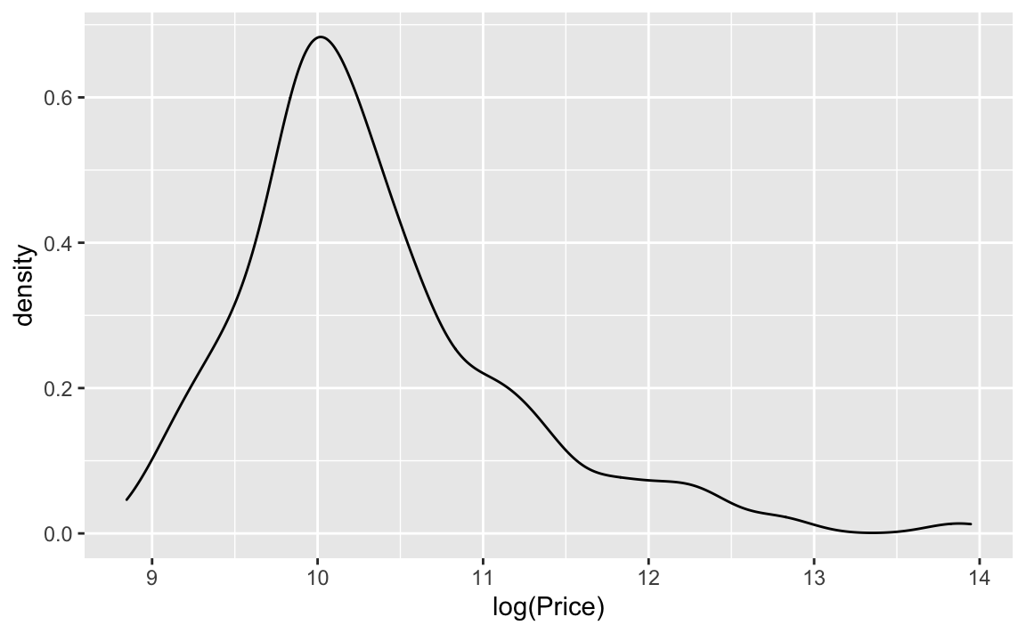

ggplot(data = TopGear,
       aes(x = log(Price),
           fill = Origin)) +
  geom_density(alpha = .5)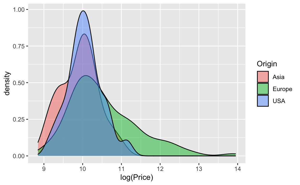

1.3 Wie ist der Zusammenhang von Preis und Beurteilung des Autos?

ggplot(TopGear,
       aes(x = Price, y = Verdict)) +
  geom_jitter()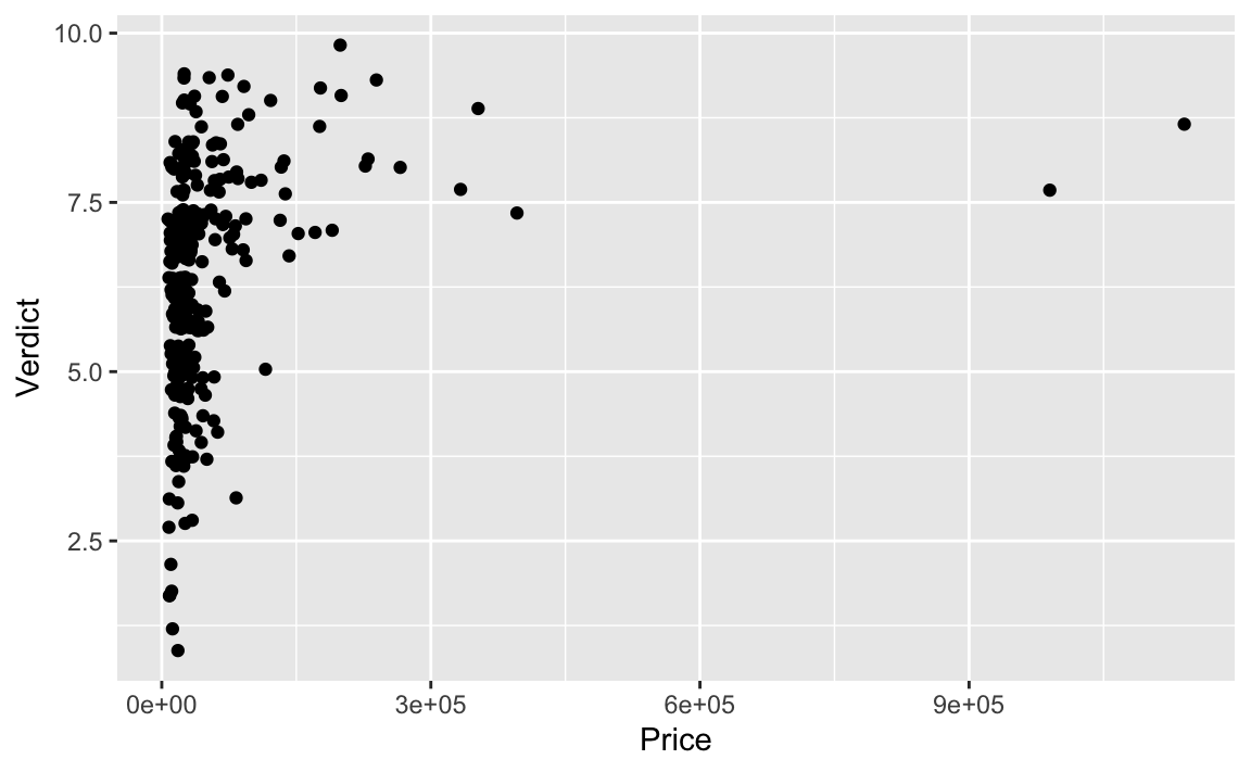

ggplot(TopGear,
       aes(x = log(Price), y = Verdict)) +
  geom_jitter()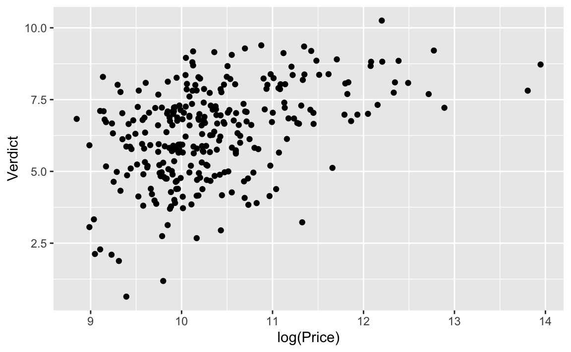

ggplot(TopGear,
       aes(x = log(Price), y = Verdict, color = Origin)) +
  geom_jitter()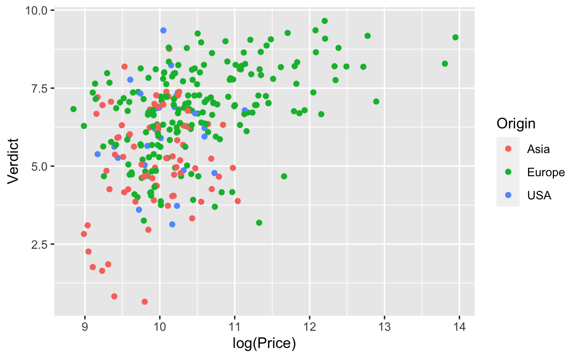

2 Wie verteilt sich das Gewicht der Autos?

ggplot(TopGear,
       aes(x = Weight)) +
  geom_density()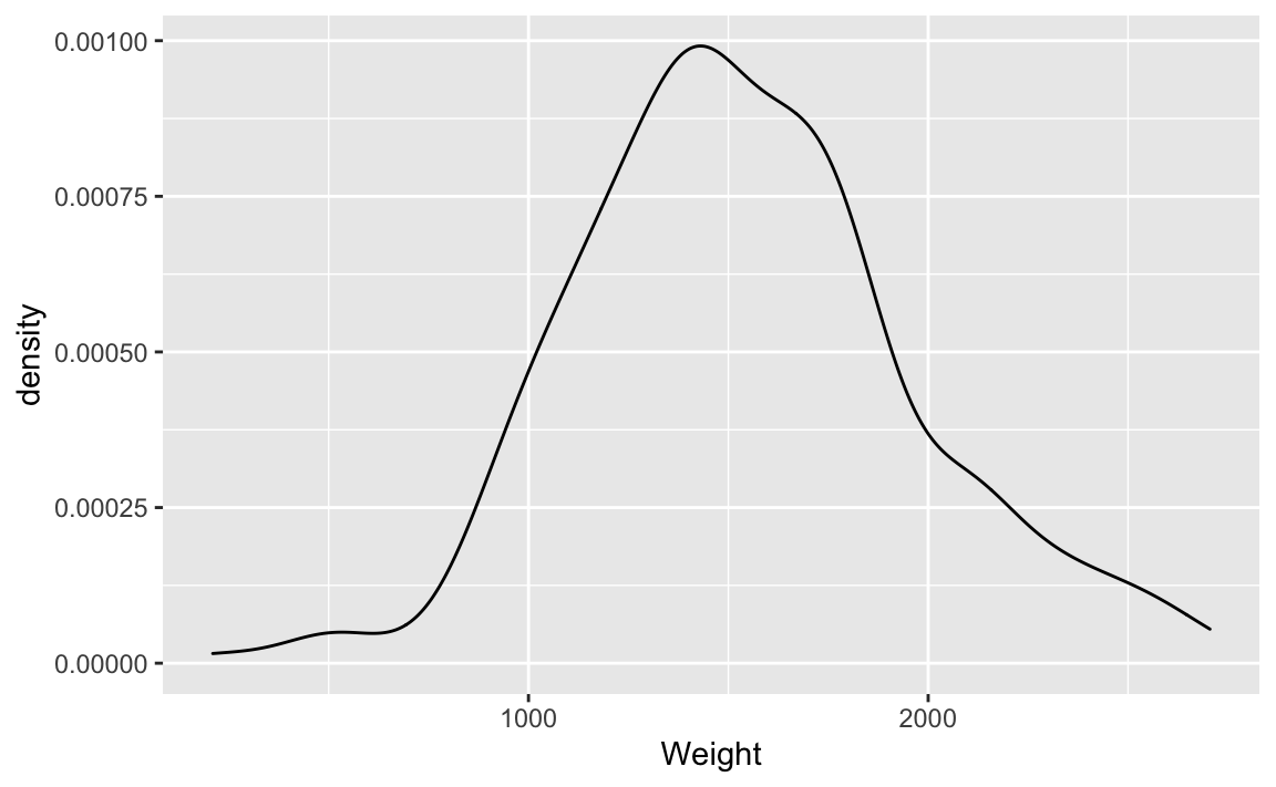

ggplot(TopGear,
       aes(x = Weight,
           fill = Origin)) +
  geom_density(alpha = .5)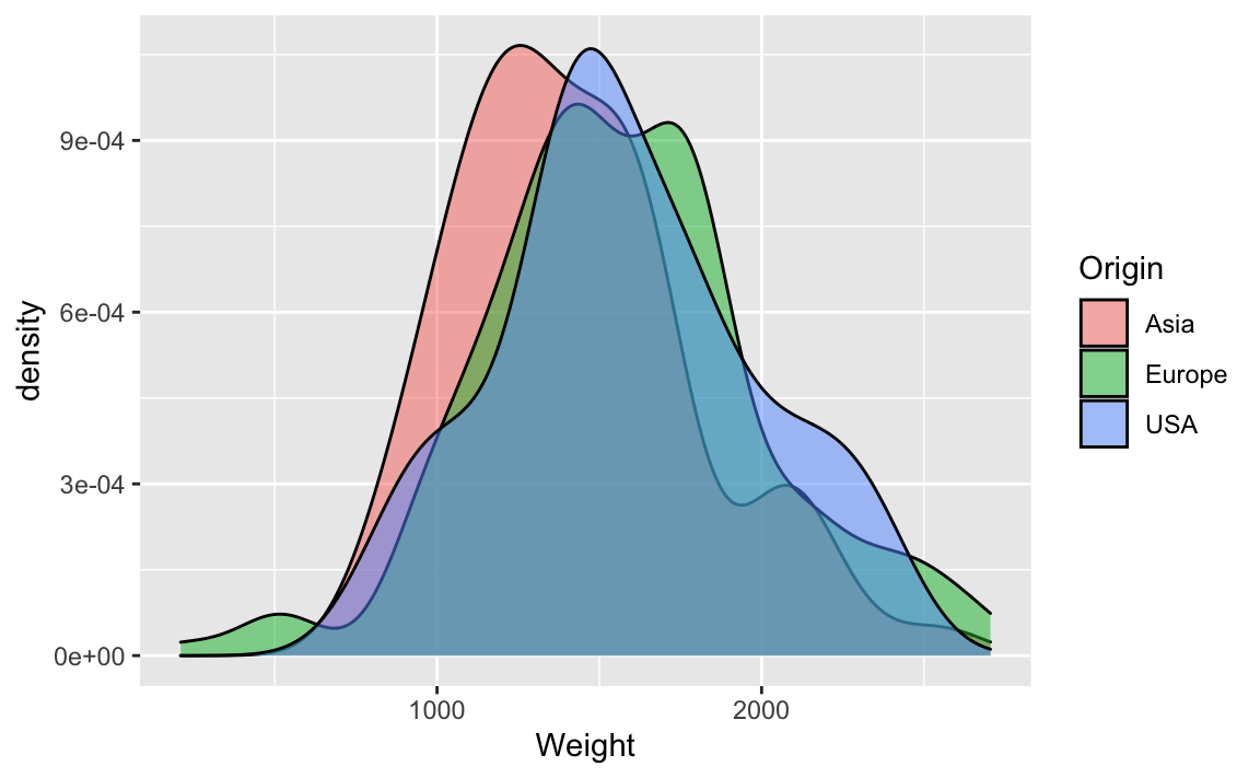

3 Hängt Gewicht mit Preis zusammen?

TopGear %>% 
  ggplot(aes(x = Weight, y = Verdict, color = Origin)) +
  geom_jitter()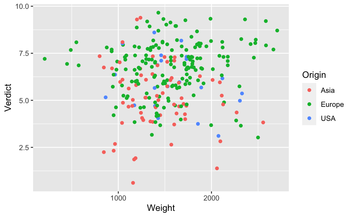

4 Wie verteilt sich die Geschwindigkeit der Autos?

ggplot(TopGear,
       aes(x = TopSpeed,
           fill = Origin)) +
  geom_density(alpha = .5)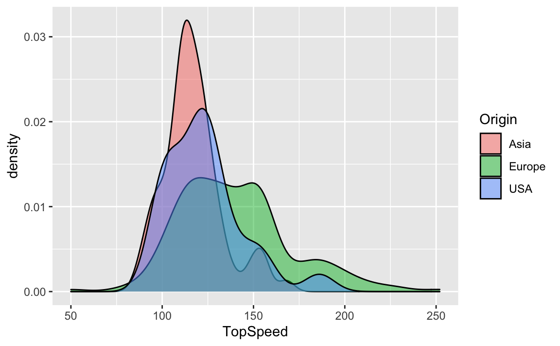

5 Hängt Preis mit Geschwindigkeit zusammen?

TopGear %>% 
  ggplot(aes(x = TopSpeed, y = log(Price), color = Origin)) +
  geom_jitter()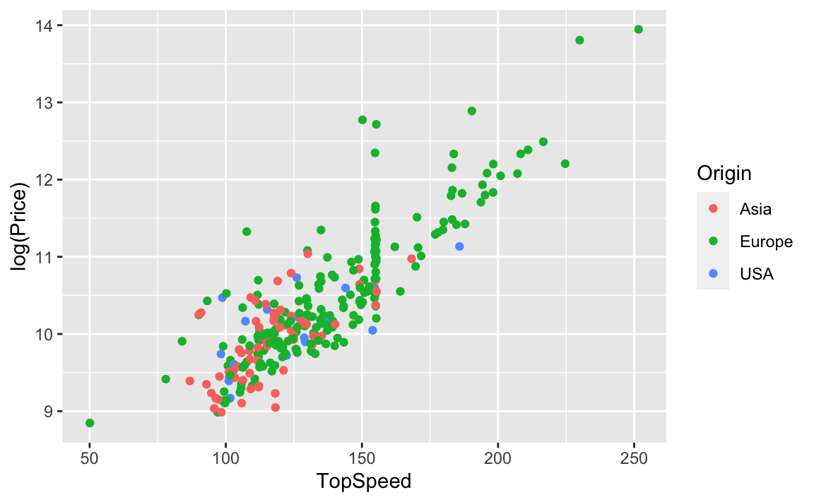

5.1 Wie hängt Geschwindigkeit mit Beurteilung zusammen?

TopGear %>% 
  ggplot(aes(x = TopSpeed, y = Verdict)) +
  geom_jitter()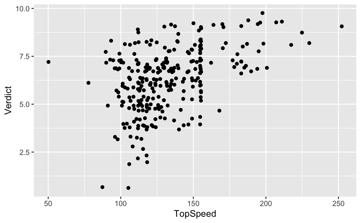

5.2 Welche Hersteller hat die meisten Autotypen?

Maker_freq <-
  TopGear %>%
  select(Maker) %>%
  count(Maker) %>%
  arrange(desc(Maker))

Maker_freq

Maker	n
Volvo	8
Volkswagen	15
Vauxhall	17
Toyota	11
Suzuki	7
Subaru	4
Ssangyong	1
Smart	1
Skoda	4
SEAT	5
Rolls-Royce	3
Renault	6
Proton	3
Porsche	4
Peugeot	10
Perodua	1
Pagani	1
Noble	1
Nissan	8
Morgan	3
Mitsubishi	5
Mini	6
Mercedes-Benz	19
McLaren	1
Mazda	3
Maserati	2
Lotus	3
Lexus	4
Land Rover	6
Lamborghini	2
Kia	8
Jeep	3
Jaguar	6
Infiniti	4
Hyundai	9
Honda	6
Ford	10
Fiat	7
Ferrari	4
Dacia	2
Corvette	1
Citroen	10
Chrysler	4
Chevrolet	7
Caterham	2
Bugatti	1
BMW	18
Bentley	4
Audi	18
Aston Martin	7
Alfa Romeo	2

Maker_Verdict <-
  TopGear %>%
  group_by(Maker)  %>%
  summarise(n = n(),
            Verdict_mean = mean(Verdict),
            Price_mean = mean(Price, na.rm = T)) %>%
  arrange(desc(Verdict_mean))

glimpse(Maker_Verdict)
#> Rows: 51
#> Columns: 4
#> $ Maker        <fct> Bugatti, McLaren, Noble, Land Rover, Lotus, Rolls-Royce,…
#> $ n            <int> 1, 1, 1, 6, 3, 3, 4, 1, 4, 6, 2, 2, 10, 19, 7, 1, 2, 18,…
#> $ Verdict_mean <dbl> 9.000000, 9.000000, 9.000000, 8.333333, 8.333333, 8.3333…
#> $ Price_mean   <dbl> 1139985.00, 176000.00, 200000.00, 48479.17, 49883.33, 30…

ggplot(Maker_Verdict, aes(x = reorder(Maker, Verdict_mean), y = Verdict_mean)) +
  geom_bar(stat = "identity") +
  coord_flip()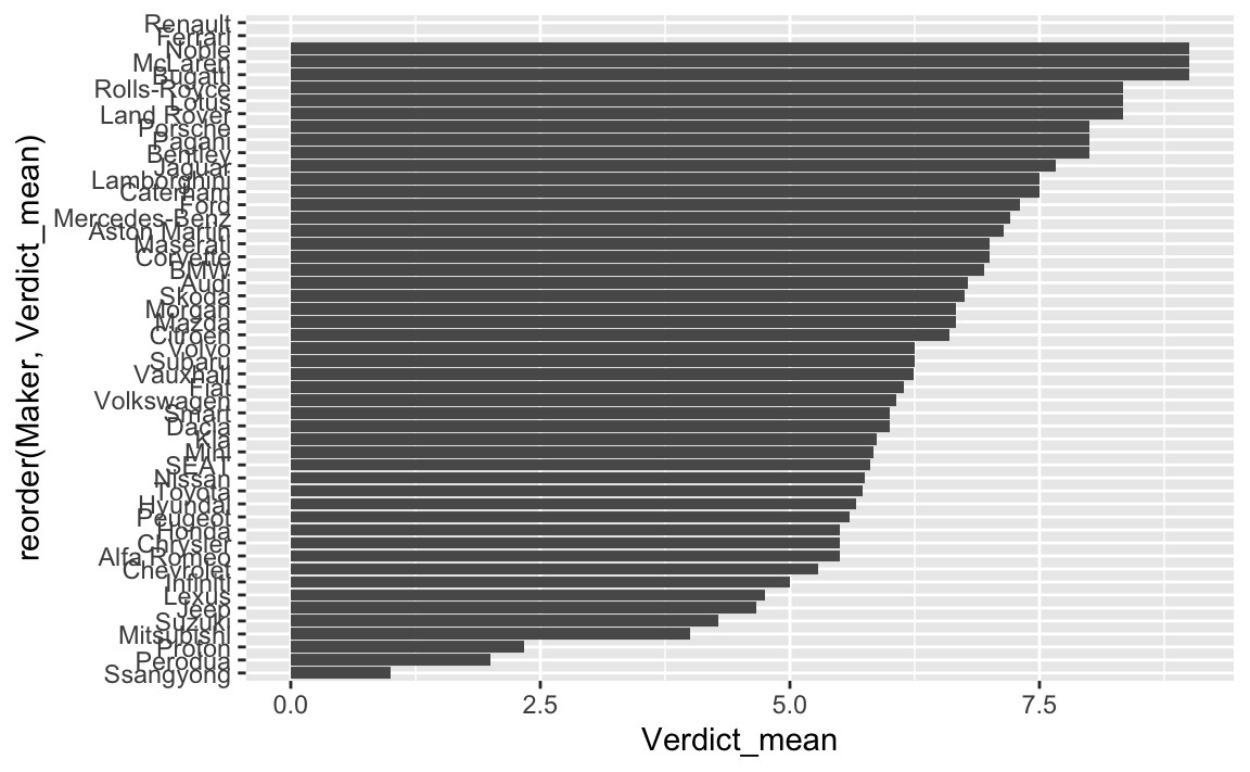

5.3 Die 10% größten Hersteller

Big10perc <-
  Maker_Verdict %>%
  filter(percent_rank(n) > .9)

5.4 Beliebtheit der 10% größten Hersteller

Maker_Verdict %>%
  filter(percent_rank(n) > .89) %>%
  ggplot(., aes(x = reorder(Maker, Verdict_mean), y = Verdict_mean)) +
           geom_bar(stat = "identity") +
  coord_flip()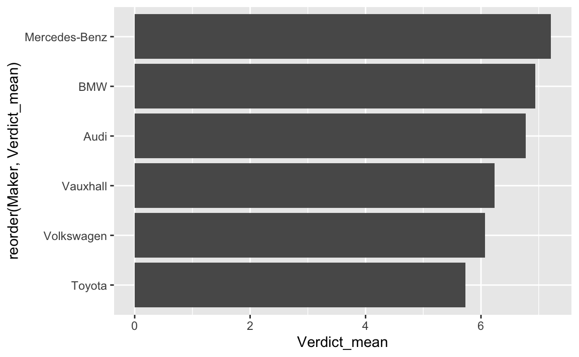

5.5 Milttlerer Preis der 10% größten Hersteller

Maker_Verdict %>%
  filter(percent_rank(n) > .89) %>%
  ggplot(., aes(x = reorder(Maker, Price_mean), y = Price_mean)) +
  geom_bar(stat = "identity") +
  coord_flip()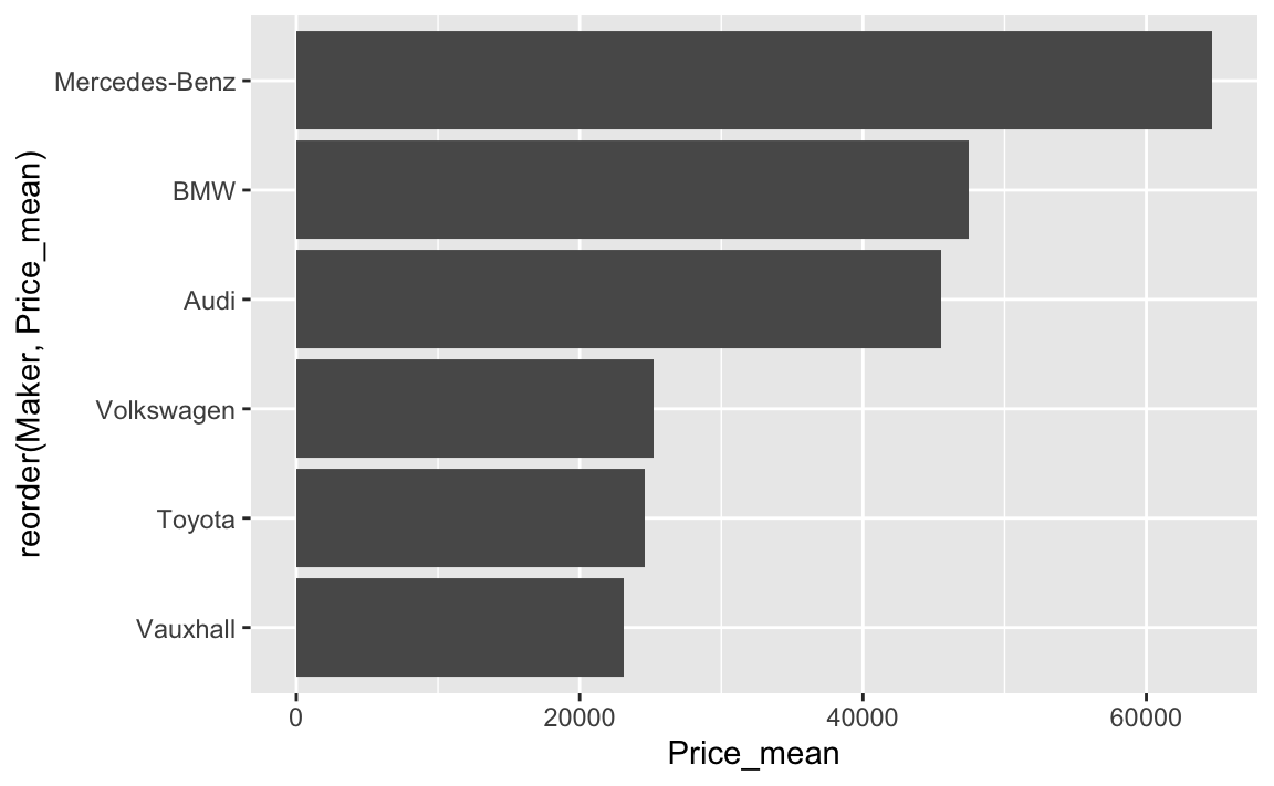

5.6 Überblick zu den 10% größten Hersteller

TopGear %>%
  filter(Maker %in% Big10perc$Maker) %>%
  skim()

Table 5.1: Data summary
Name	Piped data
Number of rows	87
Number of columns	32
_______________________
Column type frequency:
factor	19
numeric	13
________________________
Group variables	None

Variable type: factor

skim_variable	complete_rate	ordered	n_unique	top_counts
Maker	1	FALSE	5	Mer: 19, Aud: 18, BMW: 18, Vau: 17
Model	1	FALSE	87	1 S: 1, 1 S: 1, 1 S: 1, 3 S: 1
Type	1	FALSE	87	118: 1, 120: 1, 120: 1, 325: 1
Fuel	1	FALSE	2	Pet: 53, Die: 34
DriveWheel	1	FALSE	3	Fro: 33, Rea: 30, 4WD: 24
AdaptiveHeadlights	1	FALSE	3	sta: 55, no: 19, opt: 13
AdjustableSteering	1	FALSE	2	sta: 79, no: 8
AlarmSystem	1	FALSE	2	sta: 67, no/: 20
Automatic	1	FALSE	3	sta: 38, opt: 29, no: 20
Bluetooth	1	FALSE	3	sta: 59, opt: 21, no: 7
ClimateControl	1	FALSE	3	sta: 60, opt: 14, no: 13
CruiseControl	1	FALSE	3	sta: 57, opt: 19, no: 11
ElectricSeats	1	FALSE	3	no: 38, sta: 25, opt: 24
Leather	1	FALSE	3	sta: 48, opt: 22, no: 17
ParkingSensors	1	FALSE	3	sta: 57, opt: 26, no: 4
PowerSteering	1	FALSE	2	sta: 82, no: 5
SatNav	1	FALSE	3	opt: 45, sta: 33, no: 9
ESP	1	FALSE	3	sta: 82, opt: 3, no: 2
Origin	1	FALSE	1	Eur: 87, Asi: 0, USA: 0

Variable type: numeric

skim_variable	n_missing	complete_rate	mean	sd	p0	p25	p50	p75	p100	hist
Price	0	1.00	42219.54	27983.95	10435.0	23682.50	33525.0	54580.00	176895.0	▇▃▁▁▁
Cylinders	0	1.00	5.07	1.67	2.0	4.00	4.0	6.00	10.0	▁▇▃▂▁
Displacement	0	1.00	2564.13	1310.22	647.0	1598.00	1995.0	2987.00	6208.0	▆▇▅▂▂
BHP	0	1.00	235.00	130.89	68.0	141.50	204.0	272.50	571.0	▇▇▂▂▂
Torque	0	1.00	286.45	128.79	66.0	184.00	258.0	379.00	590.0	▃▇▃▃▂
Acceleration	0	1.00	8.04	2.84	3.1	5.75	7.8	9.45	16.9	▆▇▅▂▁
TopSpeed	0	1.00	138.44	20.55	93.0	123.50	139.0	155.00	196.0	▃▅▇▆▁
MPG	0	1.00	50.32	51.49	19.0	35.50	43.0	55.00	470.0	▇▁▁▁▁
Weight	13	0.85	1656.28	342.31	929.0	1430.00	1617.5	1841.50	2500.0	▂▆▇▃▂
Length	2	0.98	4575.45	343.04	3540.0	4360.00	4624.0	4877.00	5179.0	▁▂▇▇▇
Width	2	0.98	1835.28	67.01	1641.0	1786.00	1839.0	1881.00	1983.0	▁▃▇▇▂
Height	2	0.98	1493.55	140.93	1244.0	1416.00	1460.0	1578.00	1951.0	▂▇▂▂▁
Verdict	0	1.00	6.68	1.35	3.0	6.00	7.0	8.00	9.0	▂▂▆▇▇

5.7 Anzahl Modellytypen der großen Hersteller als Torte (hüstel)

ggplot(Big10perc, aes(x = Maker, y = n, fill = Maker)) + coord_polar() +
  geom_bar(stat="identity")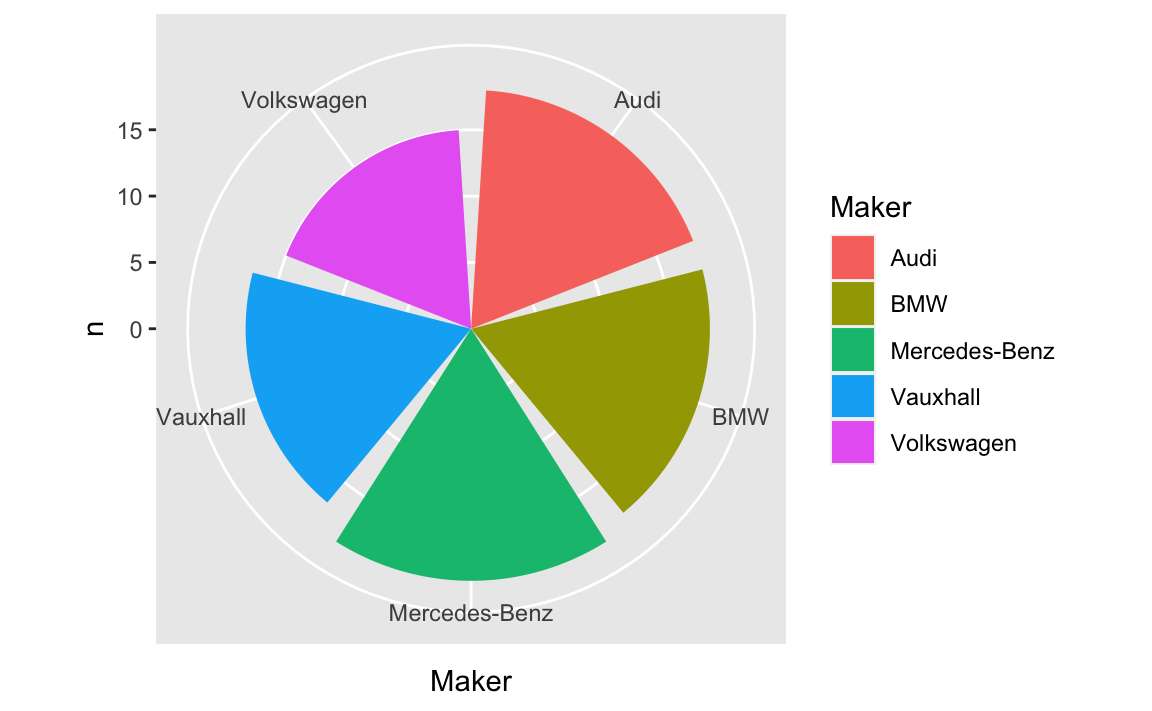

Torten stehen nicht auf dem Speiseplan…

5.8 Anzahl Modellytypen der großen Hersteller

ggplot(Big10perc, aes(x = Maker, y = n, fill = Maker)) +
  geom_bar(stat="identity") + coord_flip()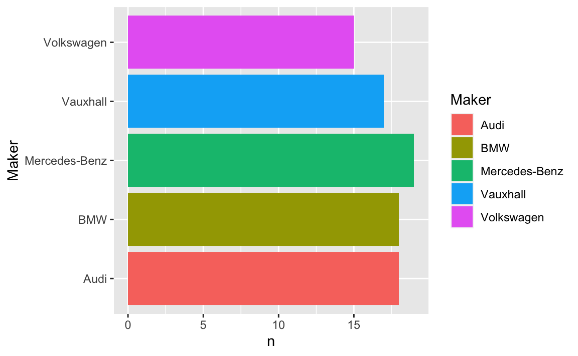

5.9 Preisverteilung der 10% größten Hersteller

TopGear %>%
  filter(Maker %in% Big10perc$Maker) %>%
  qplot(data = ., x = Price)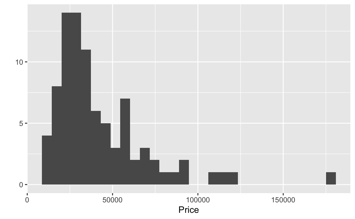

TopGear %>%
  filter(Maker %in% Big10perc$Maker) %>%
  qplot(data = ., y = Price, x = Maker)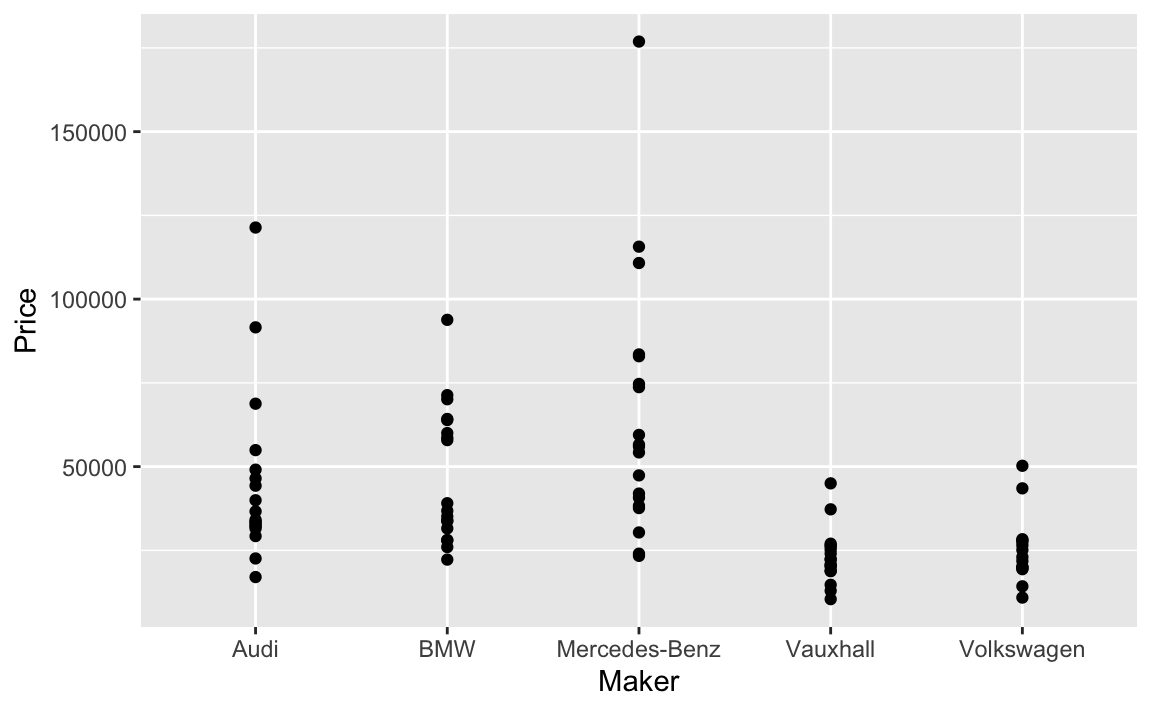

TopGear %>%
  filter(Maker %in% Big10perc$Maker) %>%
  qplot(data = ., y = Price, x = Maker, geom = "violin")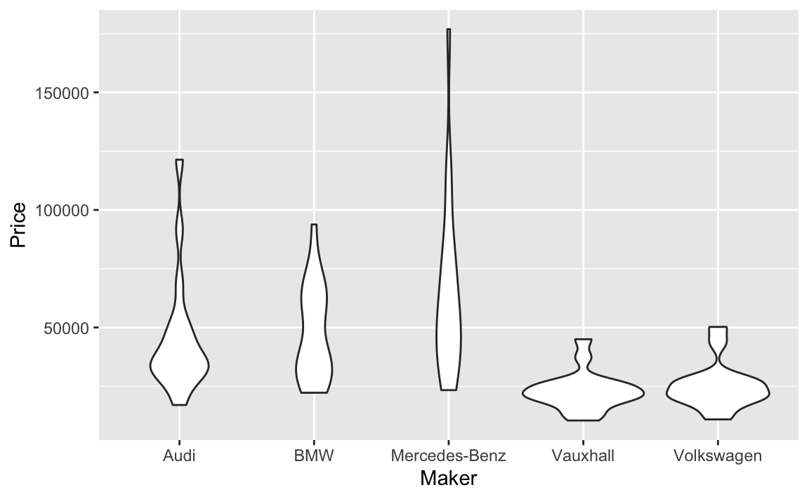

5.10 Beliebtheitsverteilung der 10% größten Hersteller

TopGear %>%
  filter(Maker %in% Big10perc$Maker) %>%
  ggplot(aes(y = Verdict, x = Maker)) +
  geom_violin()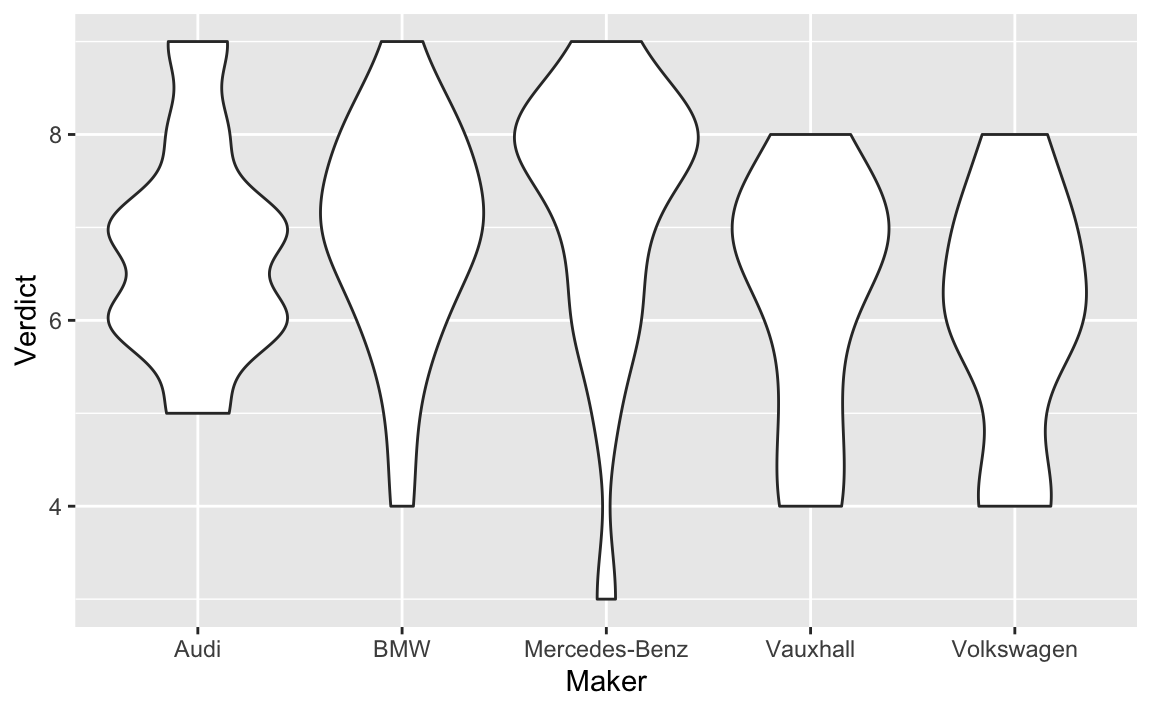

5.11 Hängt Beschleunigung mit dem Preis zusammen?

ggplot(TopGear, aes(x = Acceleration, y = Price)) + geom_hex()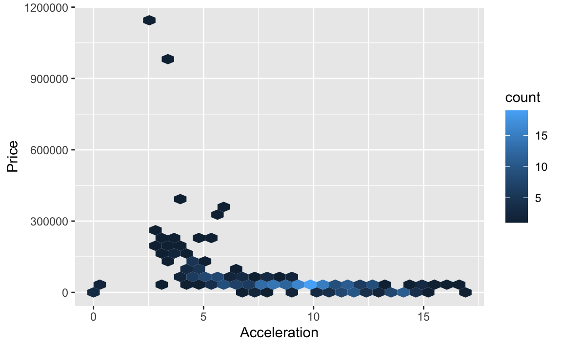

ggplot(TopGear, aes(x = Acceleration, y = log(Price))) + geom_hex()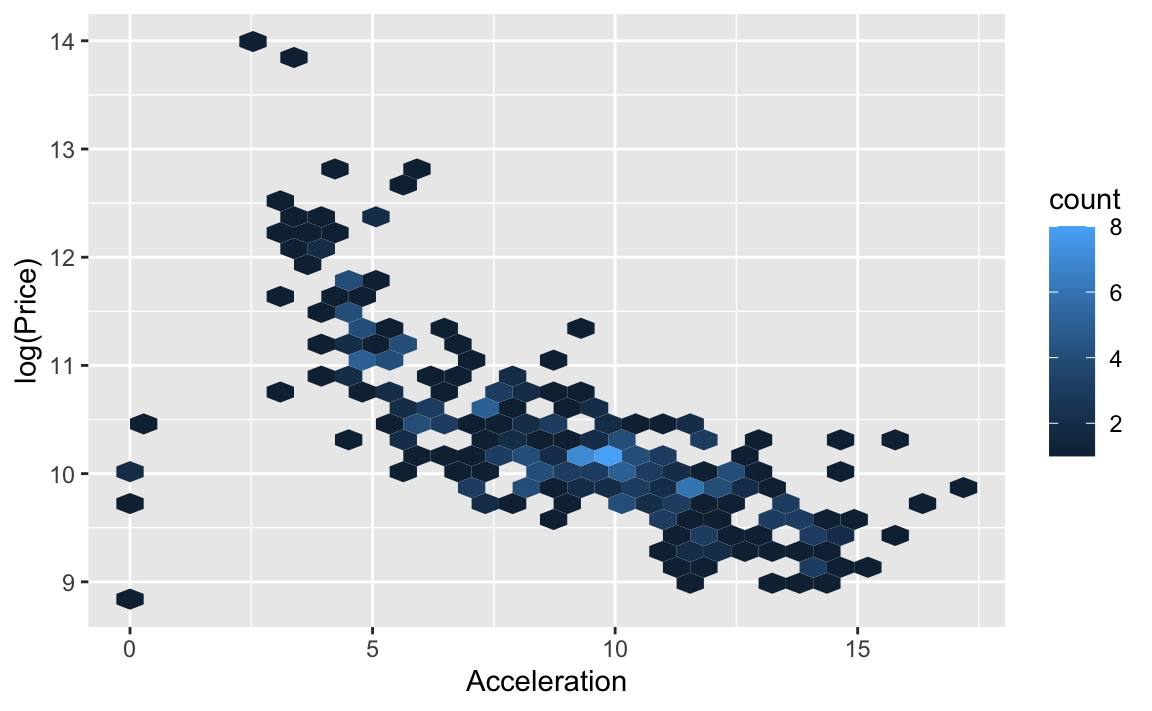

ggplot(TopGear, aes(x = Acceleration, y = log(Price))) + geom_jitter() +
  geom_smooth()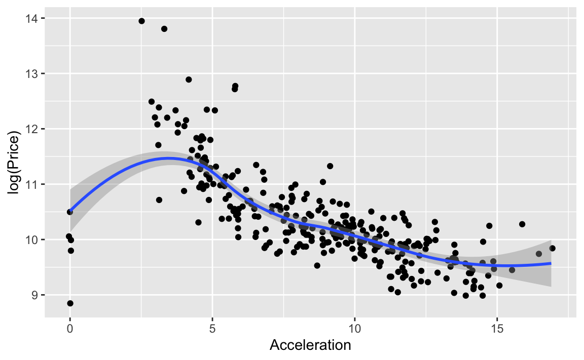

5.12 Hängt Beschleunigung mit Beurteilung zusammen? - Nur die großen Hersteller

ggplot(TopGear, aes(x = Acceleration, y = log(Price))) + geom_jitter() +
  geom_smooth()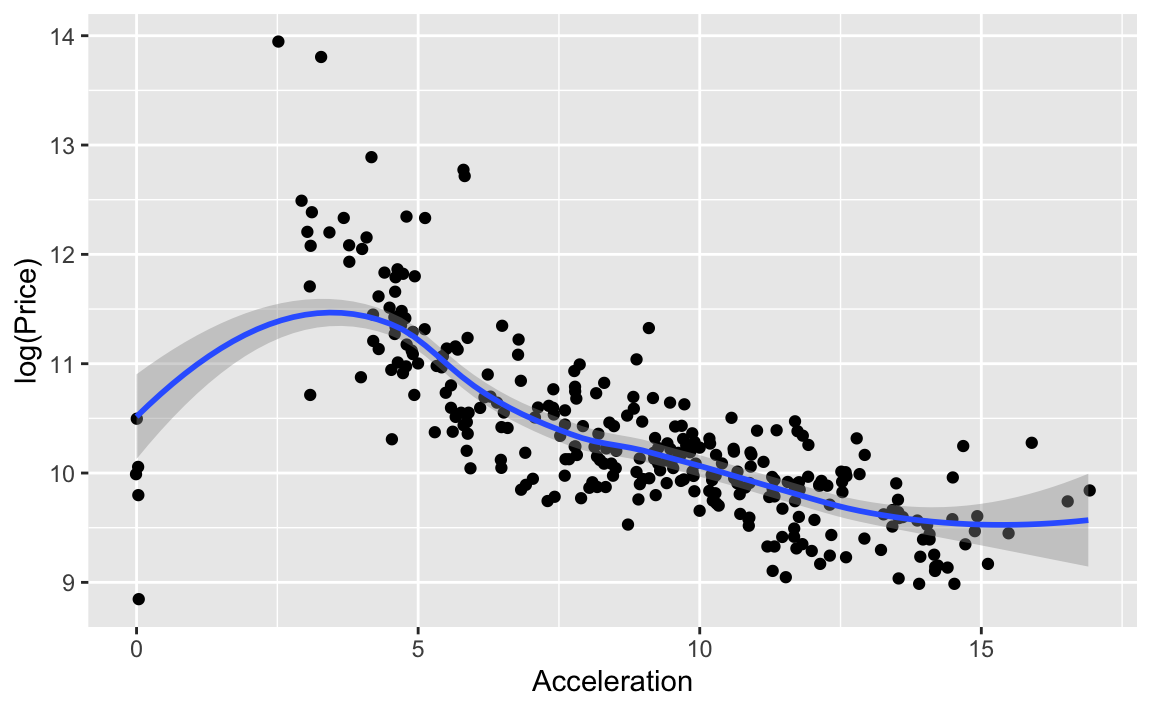

5.13 Hängt die Verwendung bestimmter Sprit-Arten mit dem Kontinent zusammen?

ggplot(TopGear, aes(x = Origin, y = Fuel, color = Origin)) + geom_jitter()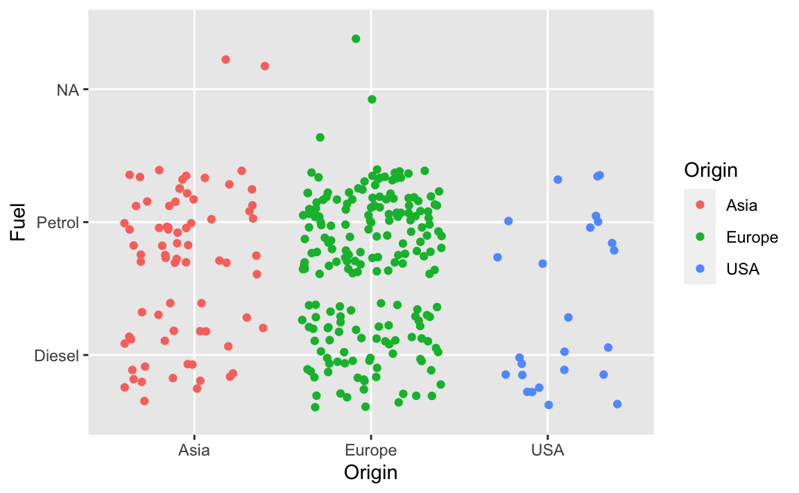

6 Reproducibility

#> ─ Session info ───────────────────────────────────────────────────────────────────────────────────────────────────────
#>  setting  value                       
#>  version  R version 4.0.2 (2020-06-22)
#>  os       macOS  10.16                
#>  system   x86_64, darwin17.0          
#>  ui       X11                         
#>  language (EN)                        
#>  collate  en_US.UTF-8                 
#>  ctype    en_US.UTF-8                 
#>  tz       Europe/Berlin               
#>  date     2021-02-11                  
#> 
#> ─ Packages ───────────────────────────────────────────────────────────────────────────────────────────────────────────
#>  package     * version     date       lib source                             
#>  assertthat    0.2.1       2019-03-21 [1] CRAN (R 4.0.0)                     
#>  backports     1.2.1       2020-12-09 [1] CRAN (R 4.0.2)                     
#>  blogdown      1.1         2021-01-19 [1] CRAN (R 4.0.2)                     
#>  bookdown      0.21.6      2021-02-02 [1] Github (rstudio/bookdown@6c7346a)  
#>  broom         0.7.4       2021-01-29 [1] CRAN (R 4.0.2)                     
#>  bslib         0.2.4.9000  2021-02-02 [1] Github (rstudio/bslib@b3cd7a9)     
#>  cachem        1.0.1       2021-01-21 [1] CRAN (R 4.0.2)                     
#>  callr         3.5.1       2020-10-13 [1] CRAN (R 4.0.2)                     
#>  cellranger    1.1.0       2016-07-27 [1] CRAN (R 4.0.0)                     
#>  cli           2.3.0       2021-01-31 [1] CRAN (R 4.0.2)                     
#>  codetools     0.2-16      2018-12-24 [2] CRAN (R 4.0.2)                     
#>  colorspace    2.0-0       2020-11-11 [1] CRAN (R 4.0.2)                     
#>  crayon        1.4.1       2021-02-08 [1] CRAN (R 4.0.2)                     
#>  DBI           1.1.1       2021-01-15 [1] CRAN (R 4.0.2)                     
#>  dbplyr        2.0.0       2020-11-03 [1] CRAN (R 4.0.2)                     
#>  desc          1.2.0       2018-05-01 [1] CRAN (R 4.0.0)                     
#>  devtools      2.3.2       2020-09-18 [1] CRAN (R 4.0.2)                     
#>  digest        0.6.27      2020-10-24 [1] CRAN (R 4.0.2)                     
#>  dplyr       * 1.0.3       2021-01-15 [1] CRAN (R 4.0.2)                     
#>  ellipsis      0.3.1       2020-05-15 [1] CRAN (R 4.0.0)                     
#>  evaluate      0.14        2019-05-28 [1] CRAN (R 4.0.0)                     
#>  fastmap       1.1.0       2021-01-25 [1] CRAN (R 4.0.2)                     
#>  forcats     * 0.5.1       2021-01-27 [1] CRAN (R 4.0.2)                     
#>  fs            1.5.0       2020-07-31 [1] CRAN (R 4.0.2)                     
#>  generics      0.1.0       2020-10-31 [1] CRAN (R 4.0.2)                     
#>  ggplot2     * 3.3.3       2020-12-30 [1] CRAN (R 4.0.2)                     
#>  glue          1.4.2       2020-08-27 [1] CRAN (R 4.0.2)                     
#>  gtable        0.3.0       2019-03-25 [1] CRAN (R 4.0.0)                     
#>  haven         2.3.1       2020-06-01 [1] CRAN (R 4.0.0)                     
#>  hms           1.0.0       2021-01-13 [1] CRAN (R 4.0.2)                     
#>  htmltools     0.5.1.1     2021-01-22 [1] CRAN (R 4.0.2)                     
#>  httr          1.4.2       2020-07-20 [1] CRAN (R 4.0.2)                     
#>  jquerylib     0.1.3       2020-12-17 [1] CRAN (R 4.0.2)                     
#>  jsonlite      1.7.2       2020-12-09 [1] CRAN (R 4.0.2)                     
#>  knitr         1.31        2021-01-27 [1] CRAN (R 4.0.2)                     
#>  lifecycle     0.2.0       2020-03-06 [1] CRAN (R 4.0.0)                     
#>  lubridate     1.7.9.2     2020-11-13 [1] CRAN (R 4.0.2)                     
#>  magrittr      2.0.1       2020-11-17 [1] CRAN (R 4.0.2)                     
#>  memoise       2.0.0       2021-01-26 [1] CRAN (R 4.0.2)                     
#>  modelr        0.1.8       2020-05-19 [1] CRAN (R 4.0.0)                     
#>  munsell       0.5.0       2018-06-12 [1] CRAN (R 4.0.0)                     
#>  pillar        1.4.7       2020-11-20 [1] CRAN (R 4.0.2)                     
#>  pkgbuild      1.2.0       2020-12-15 [1] CRAN (R 4.0.2)                     
#>  pkgconfig     2.0.3       2019-09-22 [1] CRAN (R 4.0.0)                     
#>  pkgload       1.1.0       2020-05-29 [1] CRAN (R 4.0.0)                     
#>  prettyunits   1.1.1       2020-01-24 [1] CRAN (R 4.0.0)                     
#>  processx      3.4.5       2020-11-30 [1] CRAN (R 4.0.2)                     
#>  ps            1.5.0       2020-12-05 [1] CRAN (R 4.0.2)                     
#>  purrr       * 0.3.4       2020-04-17 [1] CRAN (R 4.0.0)                     
#>  R6            2.5.0       2020-10-28 [1] CRAN (R 4.0.2)                     
#>  Rcpp          1.0.6       2021-01-15 [1] CRAN (R 4.0.2)                     
#>  readr       * 1.4.0       2020-10-05 [1] CRAN (R 4.0.2)                     
#>  readxl        1.3.1       2019-03-13 [1] CRAN (R 4.0.0)                     
#>  remotes       2.2.0       2020-07-21 [1] CRAN (R 4.0.2)                     
#>  reprex        1.0.0       2021-01-27 [1] CRAN (R 4.0.2)                     
#>  rlang         0.4.10      2020-12-30 [1] CRAN (R 4.0.2)                     
#>  rmarkdown     2.6.6       2021-02-11 [1] Github (rstudio/rmarkdown@a62cb20) 
#>  rprojroot     2.0.2       2020-11-15 [1] CRAN (R 4.0.2)                     
#>  rstudioapi    0.13.0-9000 2021-02-11 [1] Github (rstudio/rstudioapi@9d21f50)
#>  rvest         0.3.6       2020-07-25 [1] CRAN (R 4.0.2)                     
#>  sass          0.3.1       2021-01-24 [1] CRAN (R 4.0.2)                     
#>  scales        1.1.1       2020-05-11 [1] CRAN (R 4.0.0)                     
#>  sessioninfo   1.1.1       2018-11-05 [1] CRAN (R 4.0.0)                     
#>  stringi       1.5.3       2020-09-09 [1] CRAN (R 4.0.2)                     
#>  stringr     * 1.4.0       2019-02-10 [1] CRAN (R 4.0.0)                     
#>  testthat      3.0.1       2020-12-17 [1] CRAN (R 4.0.2)                     
#>  tibble      * 3.0.6       2021-01-29 [1] CRAN (R 4.0.2)                     
#>  tidyr       * 1.1.2       2020-08-27 [1] CRAN (R 4.0.2)                     
#>  tidyselect    1.1.0       2020-05-11 [1] CRAN (R 4.0.0)                     
#>  tidyverse   * 1.3.0       2019-11-21 [1] CRAN (R 4.0.0)                     
#>  usethis       2.0.0       2020-12-10 [1] CRAN (R 4.0.2)                     
#>  vctrs         0.3.6       2020-12-17 [1] CRAN (R 4.0.2)                     
#>  withr         2.4.1       2021-01-26 [1] CRAN (R 4.0.2)                     
#>  xfun          0.21        2021-02-10 [1] CRAN (R 4.0.2)                     
#>  xml2          1.3.2       2020-04-23 [1] CRAN (R 4.0.0)                     
#>  yaml          2.2.1       2020-02-01 [1] CRAN (R 4.0.0)                     
#> 
#> [1] /Users/sebastiansaueruser/Rlibs
#> [2] /Library/Frameworks/R.framework/Versions/4.0/Resources/library

YACSDA: Topgear