stan_glm_prioriwerte

Exercise

Berechnet man eine Posteriori-Verteilung mit stan_glm(), so kann man entweder die schwach informativen Prioriwerte der Standardeinstellung verwenden, oder selber Prioriwerte definieren.

Betrachten Sie dazu dieses Modell:

stan_glm(price ~ cut, data = diamonds, 
                   prior = normal(location = c(100, 100, 100, 100),
                                  scale = c(10, 10, 10, 10)),
                   prior_intercept = normal(3000, 500))

Beziehen Sie sich auf den Datensatz diamonds.

Hinweise:

• Gehen Sie davon aus, dass die Post-Verteilung von Intercept und Gruppeneffekte normalverteilt sind.

Welche Aussage dazu passt (am besten)?

Answerlist

• Es wird für (genau) einen Parameter eine Priori-Verteilung definiert.
• Für das Regressionsgewicht \(\beta_1\) sind negative Werte apriori plausibel.
• Mit prior = normal() werden Gruppenmittelwerte definiert.
• Alle Parameter des Modells sind normalverteilt.

Solution

Probieren geht über Studieren:

Die Prioris, die Stan gewählt hat, kann man sich so anschauen:

Priors for model 'm1' 
------
Intercept (after predictors centered)
  Specified prior:
    ~ normal(location = 3933, scale = 2.5)
  Adjusted prior:
    ~ normal(location = 3933, scale = 9974)

Coefficients
  Specified prior:
    ~ normal(location = [0,0,0,...], scale = [2.5,2.5,2.5,...])
  Adjusted prior:
    ~ normal(location = [0,0,0,...], scale = [34685.38,20362.28,22862.49,...])

Auxiliary (sigma)
  Specified prior:
    ~ exponential(rate = 1)
  Adjusted prior:
    ~ exponential(rate = 0.00025)
------
See help('prior_summary.stanreg') for more details

Da gilt: \(\forall i: \beta_i \sim \mathcal{N}(0, 2.5)\) (alle betas sind normalverteilt mit Mittelwert 0 und Streuung 2.5), liegt die Wahrscheinlichkeit (apriori) bei 50%, dass der Wert von _i$ negativ ist. Anders gesagt: Wir glauben zu 50%, dass der Parameter einen negativen Wert hat.

Hier sind die Modellparameter:

Parameter	Median	CI	CI_low	CI_high	pd	Rhat	ESS	Prior_Distribution	Prior_Location	Prior_Scale
(Intercept)	4357.1021	0.95	4163.48340	4549.0046	1.00000	1.002195	1306.422	normal	3932.8	9973.599
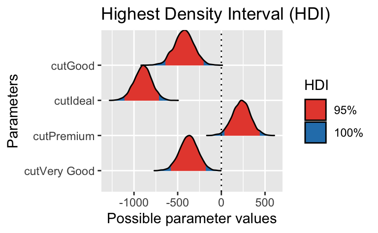
cutGood	-427.2039	0.95	-648.33634	-204.0461	1.00000	1.001761	1416.622	normal	0.0	34685.376
cutIdeal	-898.8069	0.95	-1099.13550	-701.9003	1.00000	1.001812	1313.329	normal	0.0	20362.277
cutPremium	227.0853	0.95	24.00016	430.0329	0.98675	1.001917	1282.774	normal	0.0	22862.493
cutVery Good	-375.9975	0.95	-578.22326	-171.8707	1.00000	1.002031	1387.058	normal	0.0	23922.148

Wie man sieht, sind negative Werte auch aposteriori plausibel für \(\beta_1\), cutGood:

Answerlist

• Falsch. Es gibt mehrere Parameter im Modell (Achsenabschnitt, 4 Prädiktoren, sigma)
• Wahr. Für cutGood sind negative Werte plausibel.
• Falsch. prior = normal() werden Regressionskoeffizienten in ihren Prioris definiert.
• Falsch. sigma ist in Stans Voreinstellung exponentialverteilt.

---

Categories:

• bayes
• regression