ppv-dyn1

Aufgabe

Berechnen Sie folgendes Modell (Datensatz mtcars):

mpg ~ hp

Geben Sie die Breite eines 50%-ETI an für eine Beobachtung mit einem z-Wert von 0 im Prädiktor!

Hinweise:

• Orientieren Sie sich im Übrigen an den allgemeinen Hinweisen des Datenwerks.

Lösung

Setup

library(rstanarm)
library(easystats)
library(tidyverse)

mtcars2 <-
  mtcars %>% 
  mutate(hp = standardize(hp))

Modell

m1 <- stan_glm(mpg ~ hp, data = mtcars, seed = 42, refresh = 0)
coef(m1)

(Intercept)          hp 
30.11668130 -0.06820988 

r2(m1)

# Bayesian R2 with Compatibility Interval

  Conditional R2: 0.586 (95% CI [0.378, 0.746])

Oder mit z-standardisierten Werten:

m2 <- stan_glm(mpg ~ hp, data = mtcars2, seed = 42, refresh = 0)
coef(m2)

(Intercept)          hp 
  20.096771   -4.676665 

r2(m2)

# Bayesian R2 with Compatibility Interval

  Conditional R2: 0.586 (95% CI [0.378, 0.746])

PPV

m2_ppv <- estimate_prediction(m2, data = tibble(hp = 0), ci = 0.5)
m2_ppv

Model-based Prediction

hp   | Predicted |   SE |         50% CI
----------------------------------------
0.00 |     20.11 | 4.05 | [17.44, 22.78]

Variable predicted: mpg

Visualisierung:

plot(estimate_prediction(m2))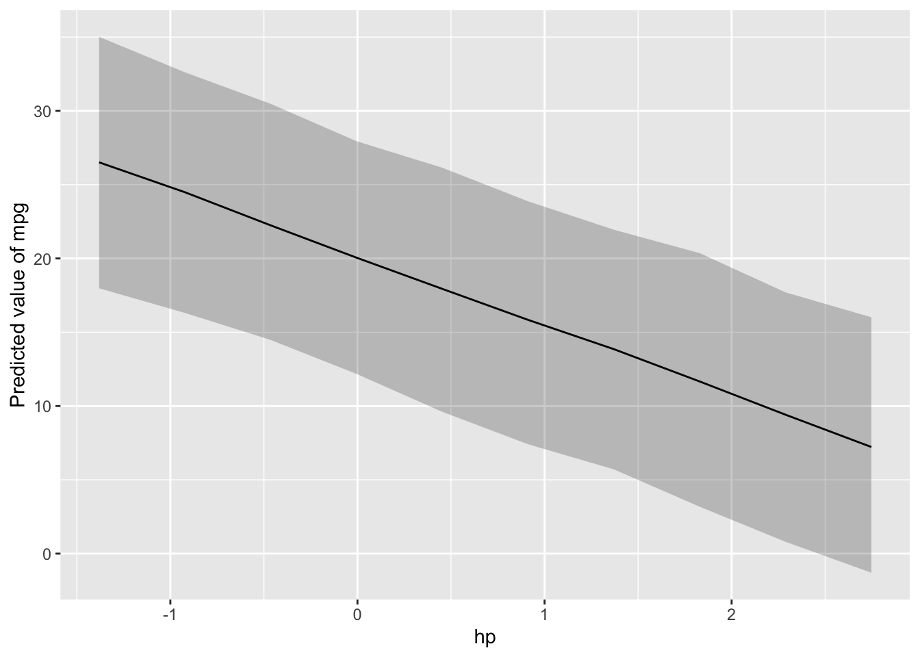

Man beachte, dass die PPV mit mehr Ungewissheit behaftet ist, als die Post-Verteilung.

plot(estimate_relation(m2))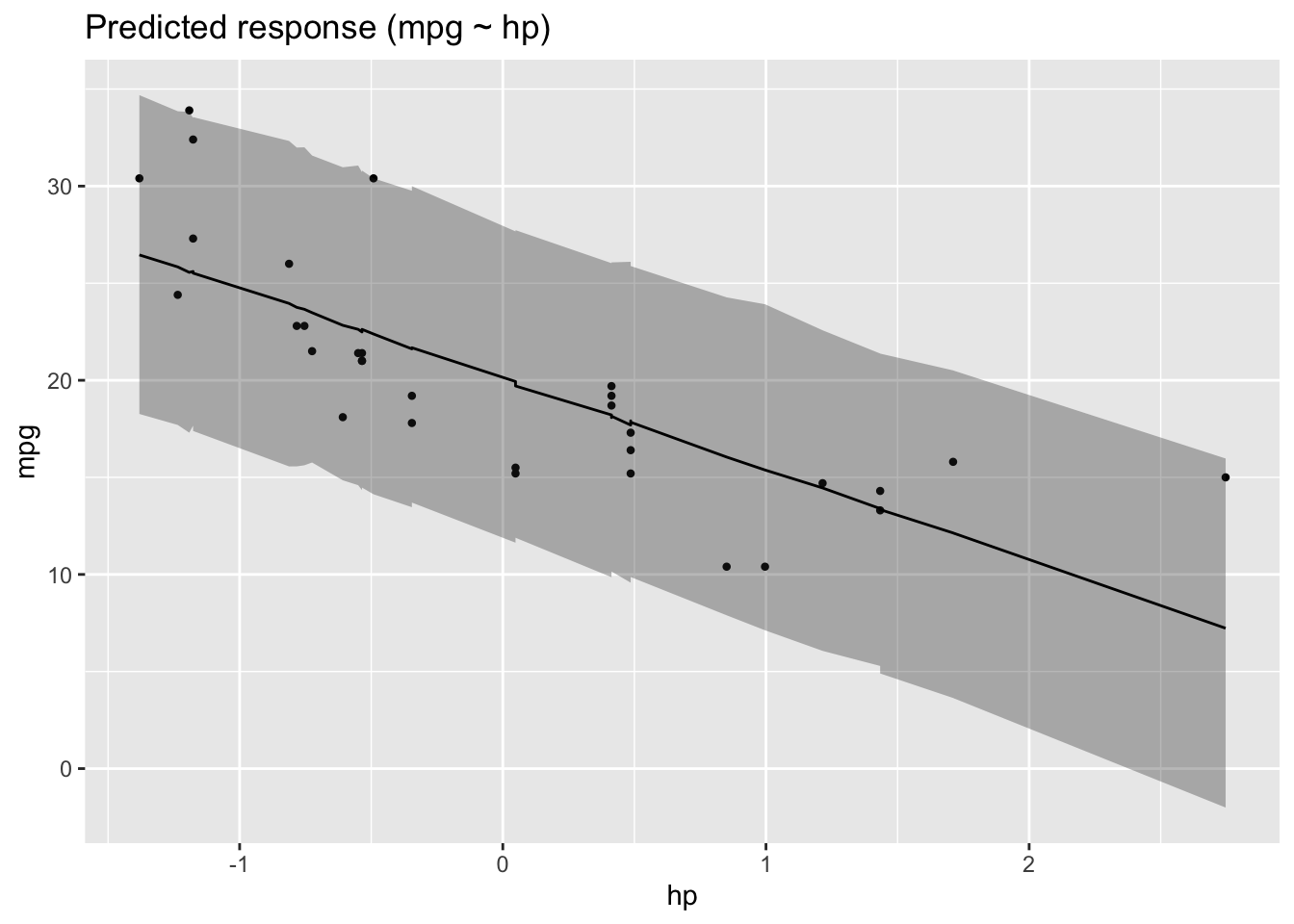

---

Categories:

• bayes
• ppv
• regression
• num