Welche Verteilung ist (am besten) geeignet, um Streuung (\(\sigma\)) zu modellieren?
Answerlist
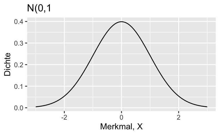
N(0,1)
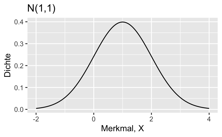
N(1,1)
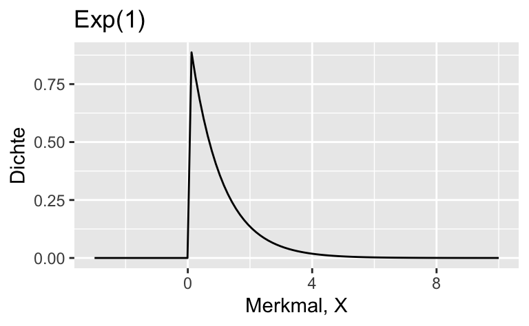
Exp(1)
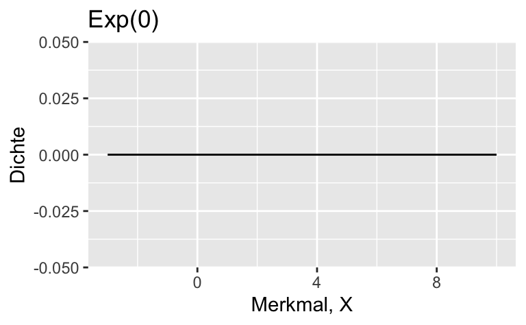
Exp(0)
Exp(-1)
Solution
Answerlist
Falsch
Falsch
Wahr
Falsch
Falsch
Da Streuung \(\sigma\) per Definition positiv ist, kommt eine Verteilung, die negative Werte erlaubt, nicht in Frage. Die Normalverteilung scheidet also aus.
Die Rate der Exponentialverteilung regelt gleichzeitig Streuung und Mittelwert. Allerdings hat \(Exp(0)\) eine unendliche Streuung, was nicht wünschenswert ist. Eine negative Rate ist für die Exponentialverteilung nicht definiert.
Normalverteilungen:
\(N(0,1)\):
\(N(1,1)\):
Exponentialverteilungen:
\(Exp(1)\):
\(Exp(0)\):
\(Exp(-1)\):
Categories:
probability
simulation
distributions
bayes
Source Code
---exname: geom-point1extype: schoiceexsolution: 64exshuffle: nocategories:- probability- simulation- distributions- bayes- qm2- qm2-pruefung2023date: '2022-11-05'title: priori-streuung---```{r libs, include = FALSE}library(tidyverse)``````{r global-knitr-options, include=FALSE}knitr::opts_chunk$set(fig.pos ='H',fig.asp =0.618,fig.width =4,fig.cap ="", fig.path ="",echo =FALSE,message =FALSE,fig.show ="hold")```# ExerciseWelche Verteilung ist (am besten) geeignet, um Streuung ($\sigma$) zu modellieren?Answerlist----------* N(0,1)* N(1,1)* Exp(1)* Exp(0)* Exp(-1)</br></br></br></br></br></br></br></br></br></br># SolutionAnswerlist----------* Falsch* Falsch* Wahr* Falsch* FalschDa Streuung $\sigma$ per Definition positiv ist, kommt eine Verteilung, die negative Werte erlaubt, nicht in Frage. Die Normalverteilung scheidet also aus.Die Rate der Exponentialverteilung regelt gleichzeitig Streuung und Mittelwert.Allerdings hat $Exp(0)$ eine unendliche Streuung, was nicht wünschenswert ist.Eine negative Rate ist für die Exponentialverteilung nicht definiert.Normalverteilungen:A)</br>$N(0,1)$:```{r}library(tidyverse)ggplot(data =data.frame(x =c(-3, 3)), aes(x)) +stat_function(fun = dnorm, n =101) +labs(y ="Dichte", x ="Merkmal, X",title ="N(0,1")```</br>B)$N(1,1)$:```{r}ggplot(data =data.frame(x =c(-2, 4)), aes(x)) +stat_function(fun = dnorm, n =101, args =list(mean =1, sd =1)) +labs(y ="Dichte", x ="Merkmal, X",title ="N(1,1)")```Exponentialverteilungen:C)$Exp(1)$:```{r}ggplot(data =data.frame(x =c(-3, 10)), aes(x)) +stat_function(fun = dexp, n =101) +labs(y ="Dichte", x ="Merkmal, X",title ="Exp(1)")```D)$Exp(0)$:```{r}ggplot(data =data.frame(x =c(-3, 10)), aes(x)) +stat_function(fun = dexp, n =101, args =list(rate =0)) +labs(y ="Dichte", x ="Merkmal, X",title ="Exp(0)")```E)$Exp(-1)$:```{r}ggplot(data =data.frame(x =c(-3, 10)), aes(x)) +stat_function(fun = dexp, n =101, args =list(rate =-1)) +labs(y ="Dichte", x ="Merkmal, X",title ="Exp(-1)")```---Categories: - probability- simulation- distributions- bayes